Comprehensive Thoughts on AI
This document aims to:
- Provide a high-level understanding of Artificial Intelligence/Machine Learning and how it works.
- Go deeper on LLMs (Large Language Models) and why they’re important.
- Help you create a prediction framework for the intelligence level of AI over time.
- Highlight the non-linear impact of AI on business, government and politics.
The second part of the document is more technical, covering a broad range of engineering topics:
- Explore what AI scaling will look like over time.
- The technical soup to nuts: from hardware to model.
The key takeaways of the document:
- AI generates non-linear effects on deployed systems/ecosystems, enabling non-linear value generation.
- Rich feedback loops in AI systems is necessary for non-linear value.
- AI systems will have a larger impact on social, economic and political than the original software revolution that started in the 80’s.
Examples of AI in Action
Let’s tour the AI technology and product landscape before trying to build an understanding of how it works. You can skip this section if you’re familiar with products and model types.
| Model Type | Tasks |
|---|---|
| Generative | Chatbots (ChatGPT, Claude etc), Video/Audio generation, code generation. |
| Object detection, tracking | Identifying/tracking objects, scenes or people in images and video. Making predictions on objects locations/trajectories. Demo |
| Speech | Cloning, tuning, speech to text, etc. Demo |
| Text Translation, Classification | Language translation, sentiment analysis etc. Demo, Demo |
| Recommendations | Search engines, YouTube recommendations, etc. Demo |
| Games, Game Theory | Game engines, combatants, etc. Demo, AlphaStar Starcraft II |
| Optimization | Compression techniques, generated code optimization, game engine up-scaling, etc. |
| Creative | Sketches to imagery, auto video generation, diffusion. Demo, Demo |
Large Language Models
Large Language Models (or LLMs) are noted for sparking widespread business and consumer interest in AI, starting with OpenAI’s ChatGPT model. There are several “frontier” LLMs, where the creators of those LLMs are pushing the frontier of intelligence in the model: Claude.ai from Anthropic and Gemini from Google. There are several models that are an intelligence generation behind, like Llama from Facebook and Mistral.ai from Mistral Labs.
Object detection, tracking and segmentation
State of the art (SOTA) object detection now includes high fidelity segmentation (bounding boxes) and the ability to track those segments across frames. Two examples of object detection models: Segment-Anything, Track-Anything

Speech
SOTA features include: speech-to-speech (OpenAI has an almost flawless implementation of speech-to-speech); speech-to-text recognition of hundreds of languages (used for YouTube closed captions); flawless text-to-speech (useful for Audiobooks etc); speech enhancement; lip reading, and more. Prime Voice AI, AutoAVSR

Generative Image Creation
Stable Diffusion, MidJourney, Microsoft CoPilot Image Creator, OpenAI Dalle3
“a portrait of an old coal miner in 19th century, beautiful painting with highly detailed face”

Generative Video Creation
NVIDIA - High-resolution video synthesis with latent diffusion models, MakeAVideo - Meta, Gen-2 Runway (StableDiffusion text to video):
“animated scene features a close-up of a short fluffy monster kneeling beside a melting red candle. the art style is 3d and realistic, with a focus on lighting and texture. the mood of the painting is one of wonder and curiosity”

Generative Game World Creation
Tencent built “GameGen-O” an AI that generates open-world games from text prompts:

Ranking and Recommendation
Most popular mobile and web apps are utilizing AI to predict what you’re interested in. The “feed” that is generated for Facebook, Instagram, TikTok etc, is unique to you, where a AI model is trained to optimize for your engagement and time spent. The better the AI is able to predict what you’re interested in, the longer you stay on the app.
Combination of Multiple Model Types
Self driving cars are an example of multiple multiple model types (image, object recognition, route planning, etc) being aggregated together to solve for a complex task like driving a car in a dynamic environment: Waymo - self driving cars
The best online places to see where machine learning model innovation is happening are:
- Hugging Face - Open Source/Downloadable Models
- Two minute papers YouTube Channel - understand new ML model research quickly.
- Reddit /r/MachineLearningNews
The basics of how ML works
Now that we’ve had a look at the top-down capability of machine learning/AI from a model and product perspective, we will start the journey to understand the basics of how machine learning works under the hood.
What is an ML Model?
There are well articulated definitions of what machine learning models are on the Internet, so I’ll say that models are essentially a piece of software that takes data as an input, and makes a prediction as an output in a domain we care about. Models are trained by looking at lots of input examples, trying to guess the output, and when there is error, the model updates itself to be less erroneous next time. Given enough examples, the model will be more precise, and hopefully general enough to give accurate predictions on input it has not seen in training.
This concept is unlikely a surprise, as we’ve been using “machine learned” models in tools like Excel for years. And ironically, one of the easiest Excel modeling techniques, linear regression, is the fundamental building block for how machine learning works in the large.
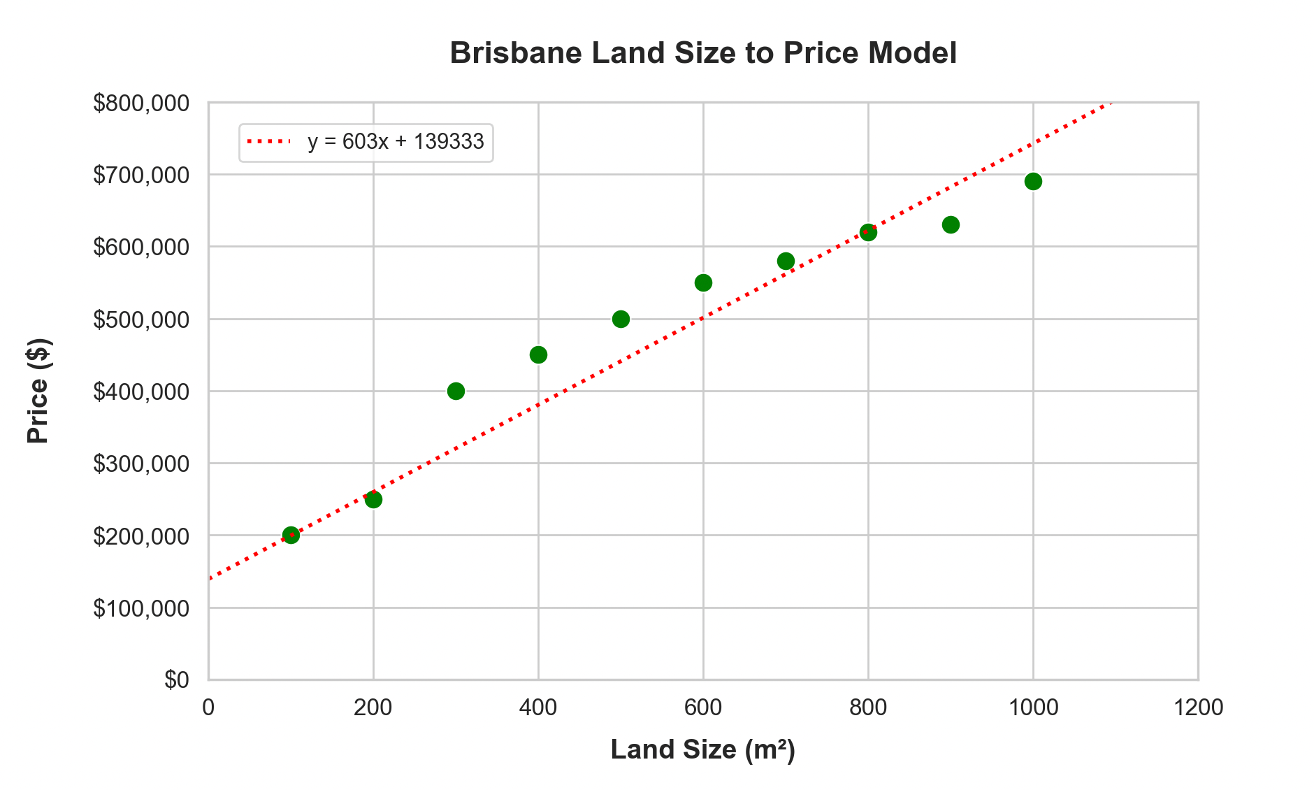
A quick recap of linear regression: We’ll build a simple linear regression model to predict house prices. Let’s take some synthetic historical house price data, which I’ve plotted below (x axis is land size in square meters, and the y-axis is the price the house sold for):
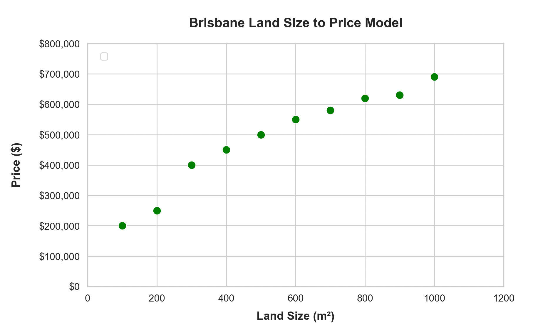 Asking Excel to generate a Linear Regression model with a couple of clicks gives me a nice red line, and a function representing the linear model:
y = 603x + 139333Where y is the house price prediction, x is the land size input and the 139333 is the y intercept.
 The slop intercept form of the linear equation above is
 y = mx + b, and has two parameters: m and b. m represents the slop of the line and b determines where the line is positioned vertically on the y-axis. These two parameters form the crux of the model.
We can now ask the model for its prediction on what the price would be for a Brisbane house given a previously unseen land size of 1095 square meters:
$799,618 = 603 * 1095 + 139333While Excel uses linear regression to figure out the best model, the machine learning world does something different:
- it starts with random numbers for all the parameters in the model
- it checks to see how good a fit that model is to the data and calculates the “error” or “loss” with respect to the data
- it adjusts the parameters of the model to make the “error” or “loss” be less error prone
- repeat steps 2 through 4 until the error is really small
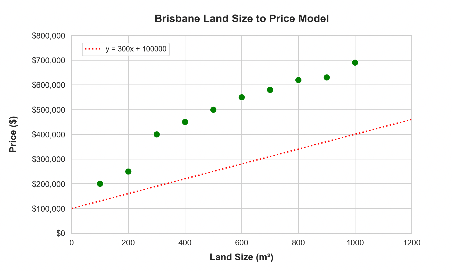
Let’s try:
price = random_p1() * land_size + random_p2()So for random_p1(), let’s assume it generated 300 as its random starting point, and 100,000 as random_p2():
Not terribly close to reality, so let’s bump the random_p1() and random_p2() numbers up, so that line gets a little steeper: y = 400 * land-size + 150000
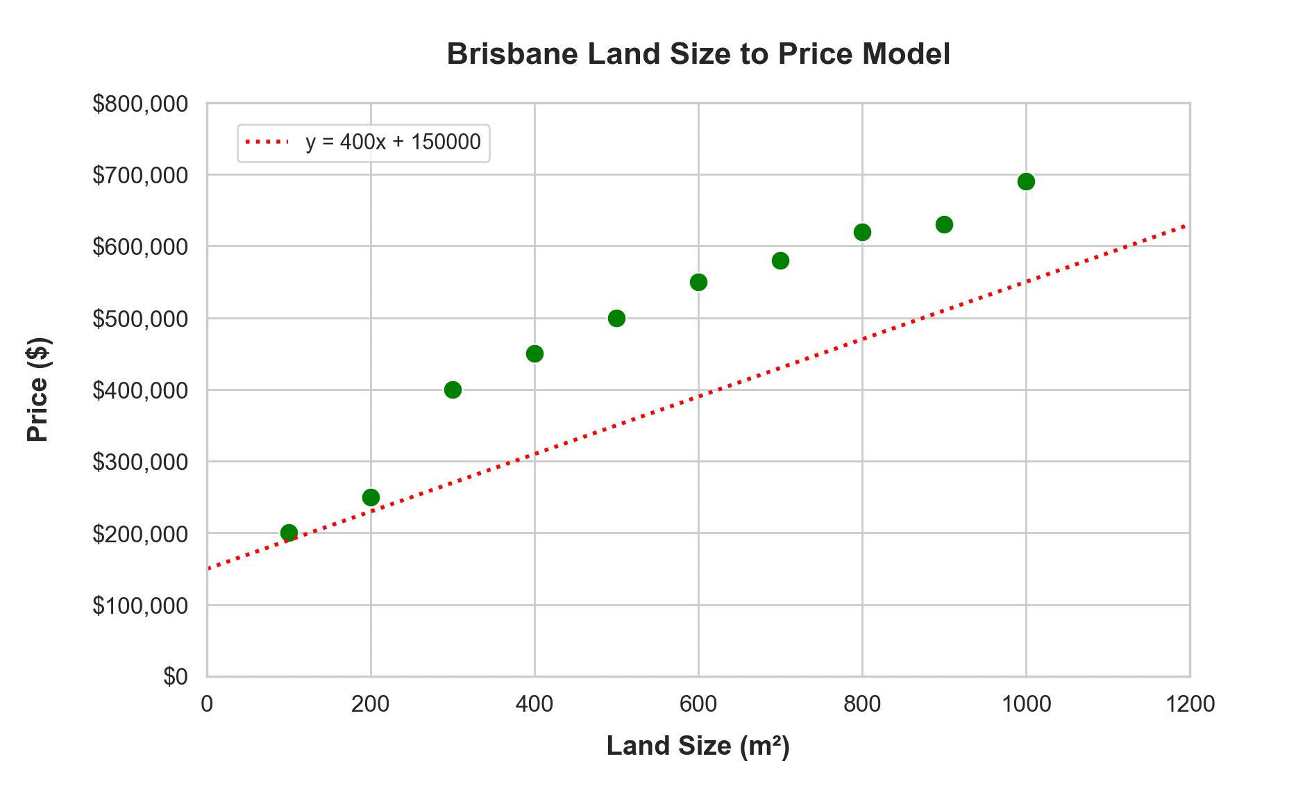 Better!
Now we’re going to repeat the “tuning” of those two parameters until the line has the least amount of “error”:
m = 300 -> 400 -> 550 -> 650 -> 610 -> 603
b = 100000 -> 150000 -> 140000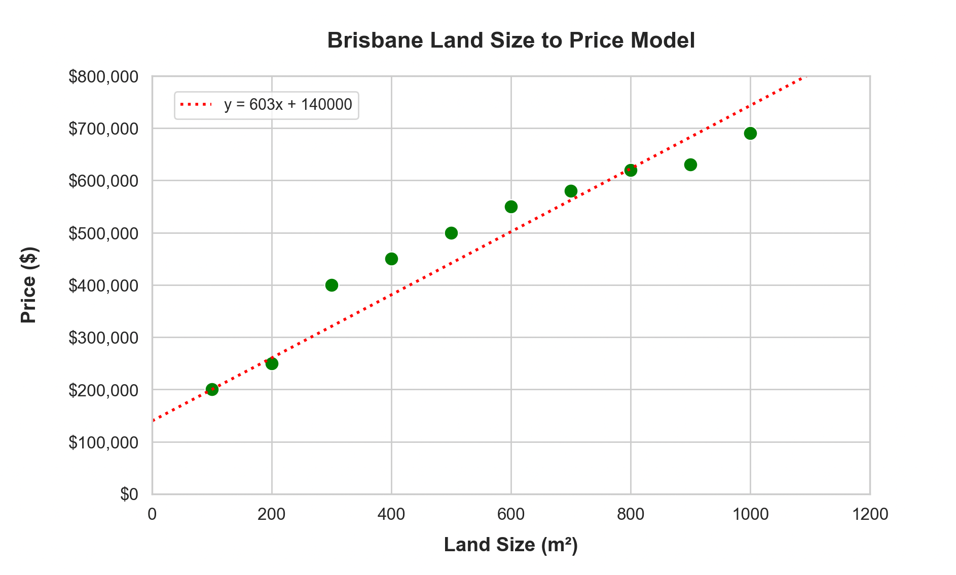
And that’s it. The machine has learned the most appropriate variables with the least amount of error are “603”, and “140000” such that price = 603 * land-size + 140000.
Before we move on, let’s go through the vocabulary definitions as they relate to machine learning for the example we’ve just seen:
- The initial number we used for random_p1() and random_p2() to adjust the slope of the line and the y-intercept, in ML terms that’s called a “parameter” or “weight”. (In Linear Regression terms, it’s call the coefficient). Parameters or weights are the “heart” or “intelligence” of the model.
- The “x” axis variable (Land Size) is called an “input parameter”. It’s the thing we give the model to make a prediction on.
- The loop of:
- Create a model with “parameters”
- Run data through the model and calculate the error
- Bump the “parameters” closer to ensure a less erroneous fit for the data we’ve seen
- This is called the “training loop”.
Two parameter models like the one we’ve built above can only generate straight lines (y-intercept and slope), which isn’t terribly useful particularly when we have data that is non-linear, like:
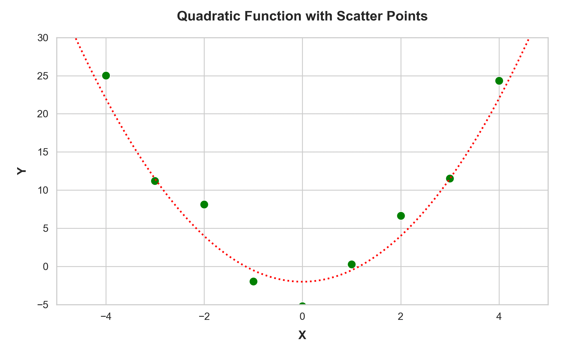 and isn’t terribly useful if you need to have many input parameters to describe the thing you care about (perhaps you want more than just land size, you want age of the house, bedrooms, bathrooms and so on).
So we need a way to (1) add more input variables, and (2) ensure we can capture any non-linearity in the model.
From one parameter to many
Scaling this to multiple input parameters is as simple as extending our linear equation to be a multivariate linear model in the form:
$$
\begin{aligned}
y = P_1x_1 + P_2x_2 + … + P_nx_n \newline
\end{aligned}
$$
There are multiple P or parameters, multiple x, which are the inputs (or input parameters), and y which is the predicted result, or thing we’re trying to learn. The training loop above still applies, we’re going to be nudging a lot more parameters in order to reduce the error now. This form however, is still insufficient to capture the non-linearity of the parabola example above (a quadratic function, while having more parameters, also uses an exponential term to represent the non-linear curve: f(x) = ax^2 + bx + c).
To get both many input-parameters, and a general way to create non-linear models that capture very complex relationships, “neural networks” were born, and they stand mostly on the shoulders of that multivariate linear equation above.
Neural Networks
You may have seen some diagrams of Neural Networks, or Deep Neural Networks. These diagrams are a graphical representation of a much larger calculation that uses the multivariate linear equation above as its fundamental building block:
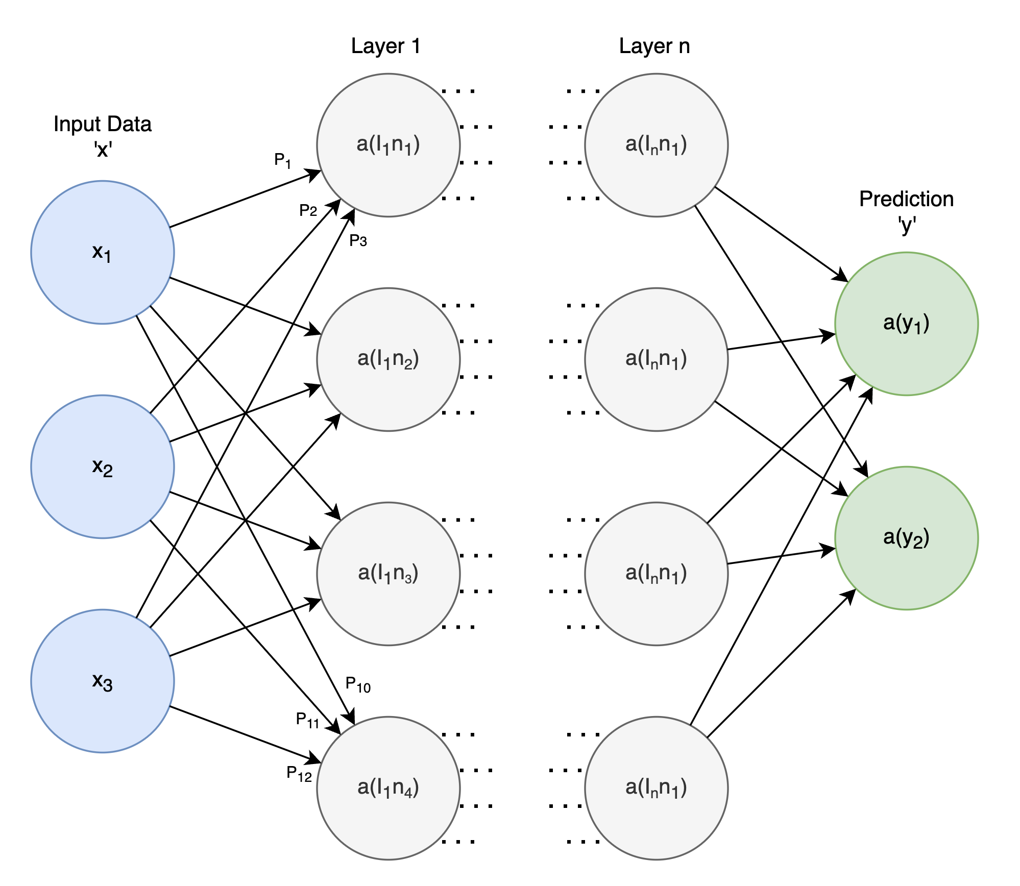
The high level view:
- Each of those grey circles are “neurons”.
- Each neuron has a set of “parameters”. The number of parameters is determined by the number of incoming connections it has from neurons on its left.
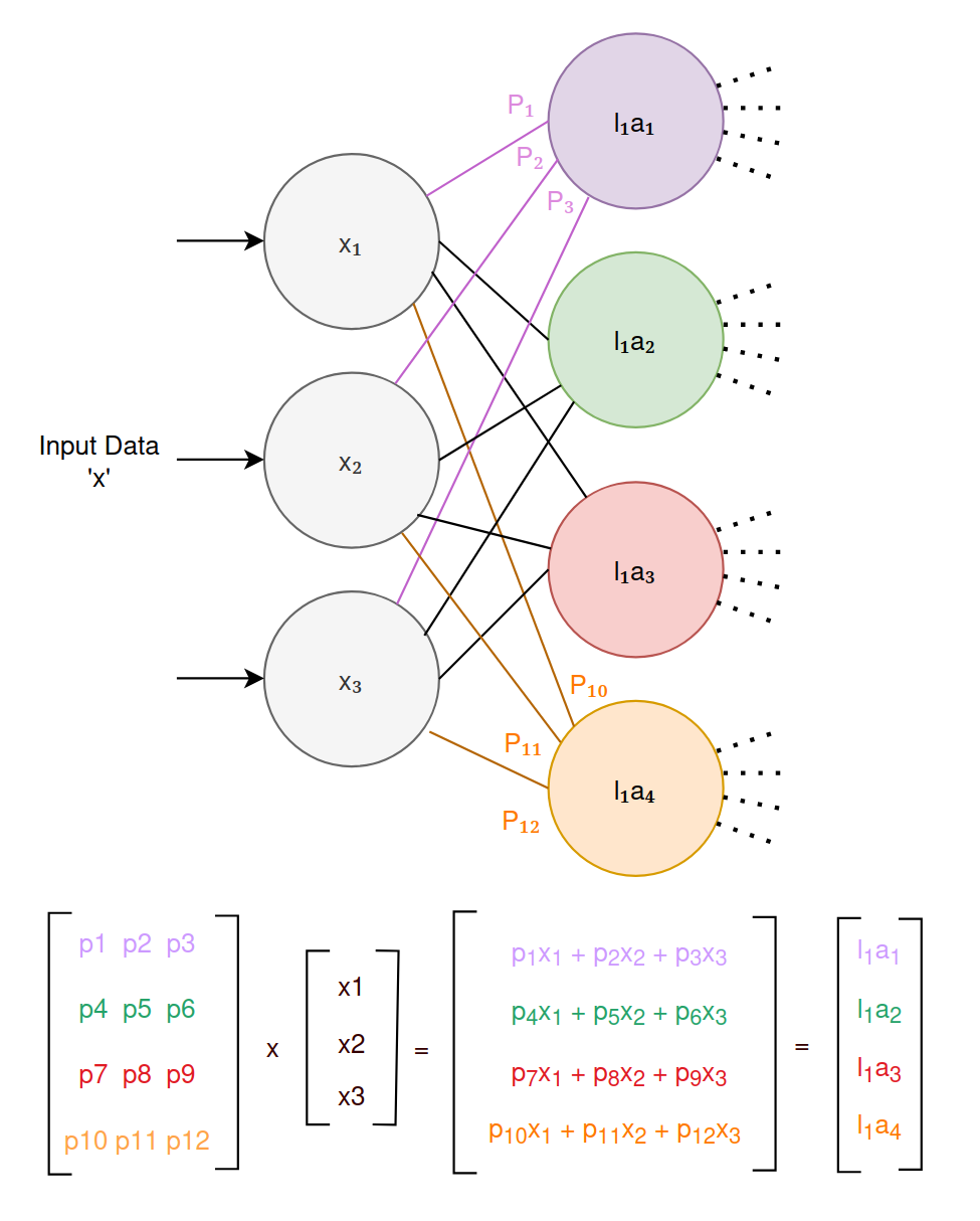
- The neuron performs two calculations, before passing the result forward via the connections to other neurons on its right.
- Linear Combination: The first calculation is the multivariate linear equation we saw above, where input data is multiplied by parameters and summed: $$ \begin{aligned} l_1n_1 = P_1x_1 + P_2x_2 + P_3x_3 \newline \end{aligned} $$
- Activation Function: The second calculation applies an “activation function”, which introduces non-linearity to the model. The activation function aaa is applied to the result of the linear combination. For example, using the sigmoid activation function, this can be written as: $$ \begin{aligned} a(l_1n_1) = sigmoid(P_1x_1 + P_2x_2 + P_3x_3) \newline \end{aligned} $$ The activation function, such as the sigmoid function, helps the neuron to produce non-linear outputs, enabling the neural network to learn more complex patterns. The sigmoid function looks like:
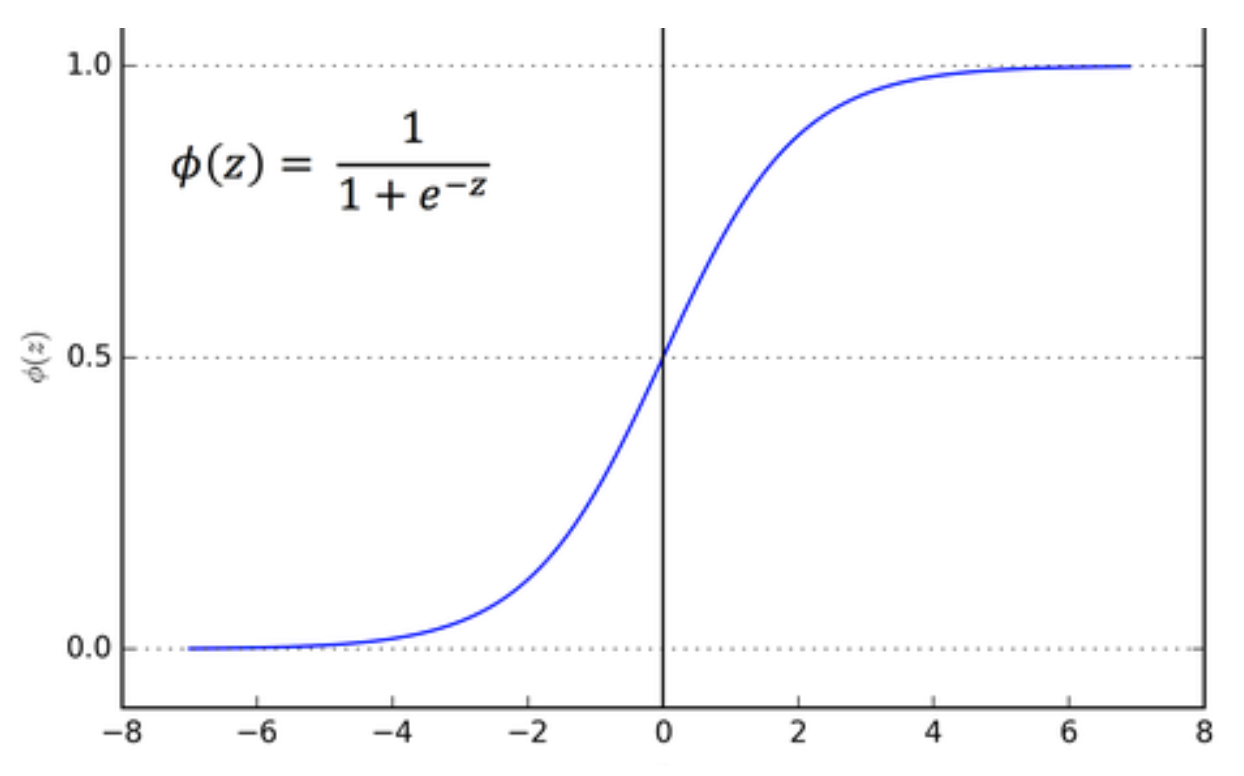
Don’t let the math symbols worry you. Just think of every neuron computing the ‘y =’ multivariate linear equation from above, and then applying a function that generates non-linearity to the result. We take data in, multiply them by parameters, send them through the activation, and produce a result for the next neuron.
We have this fancy visualization of a neural network above, because it abstracts away the rather large and complicated equation or “model” that it represents:
$$ \begin{align*} \text{Layer 1:} \newline &a(l_1n_1) = sigmoid(P_1x1+P_2x_2+P_3x_3) \newline &a(l_1n_2) = sigmoid(P_4x1+P_5x_2+P_6x_3) \newline &a(l_1n_3) = sigmoid(P_7x1+P_8x_2+P_9x_3) \newline &a(l_1n_4) = sigmoid(P_{10}x1+P_{11}x2+P{12}x_3) \newline \newline \text{Layer 2:} \newline &a(l_2n_1) = sigmoid(P_1l_1n_1 + P_2l_1n_2 + P_3l_1n_3 + P_4l_1n_4) \newline &a(l_2n_2) = sigmoid(P_5l_1n_1 + P_6l_1n_2 + P_7l_1n_3 + P_8l_1n_4) \newline &a(l_2n_3) = sigmoid(P_9l_1n_1 + P_{10}l_1n_2 + P_{11}l_1n_3 + P_{12}l_1n_4) \newline &a(l_2n_4) = sigmoid(P_{13}l_1n_1 + P_{14}l_1n_2 + P_{15}l_1n_3 + P_{16}l_1n_4) \newline \newline \text{Output Layer:} & \newline &a(y_1) = sigmoid(P_1l_2n_1 + P_2l_2n_2 + P_3l_2n_3 + P_4l_2n_4) \newline &a(y_2) = sigmoid(P_5l_2n_1 + P_6l_2n_2 + P_7l_2n_3 + P_8l_2n_4) \newline \end{align*} $$
Making the Neural Network “Fit”
Just like the original Brisbane Land Size to Prices model, where we “nudged” the two parameters of the model in the correct direction depending on how much “error” the model produced, we do the exact same thing here for neural networks:
- pass in the input data, perform the calculation for layer 1, layer 2 and the output layer, get the result from the output layer (a(y1), a(y2))
- calculate the difference between the data we have to give us the “error” in the model
- nudge all the parameters (in this case, there are 36 parameters total) in a particular direction to reduce the error
- rinse and repeat until the error is low
The more neurons, parameters, and layers there are, the more “non-linearity” and space for the model to learn and fit the data properly. You can imaging that the result of the neural network learning process is a really strange squiggly line in ’n’ dimensions of space (i.e more than three, which is easy to visualize) which properly represents a general model of the data we care about.
And with that, we’ve just learned that you can go from a single line linear regression ‘fit’, to a non-linear fit by just composing together the same basic linear equation over and over and over again.
Input and Output Data Representation
The “input data”, or “input layer”, is always encoded as a number, so a question that regularly comes up is: “how are images, video, documents etc, represented as numbers in the input layer”.
They’re always converted to their numeric representation, and its just a case of learning what the best numeric representation is for the given data:
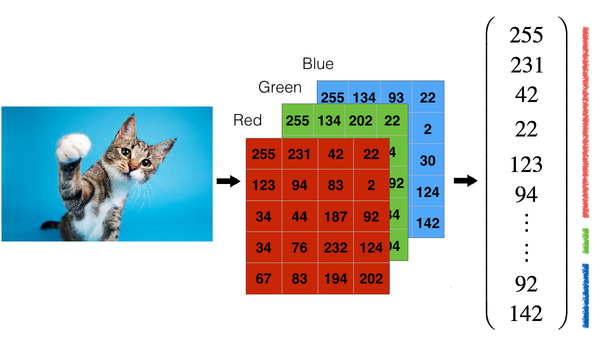 Here, every pixel of the cat image is converted to it’s red, green, blue value and those values are used in the input layer. This implies that big images with tens of thousands of pixels, will be fed to a neural network model that has tens of thousands of input neurons, and may require tens of millions of parameters to allow the model to learn something about the image! The concept is the same for video, text, and so on. Everything is converted to a number and fed in to that first “input layer”.
Text for example, can be encoded using a simple character to number encoding:
a = 1.0b = 2.0c = 3.0- and so on
Output layers (or the prediction layer) can represent text, images, video and so on in the same way.
We could build a neural network model that takes an image as an input, and produces an inverted color version of the same picture as its output, like below:

The process to build this model is the same as what we’ve seen already:
- Get a big set of examples of images: both the input image and example outputs (the inverted images)
- Start with a neural network that has random parameters
- Encode each image into a numeric representation, pixel by pixel
- Feed those images to the neural network
- See how close the output layer is to the example inverted image outputs
- Nudge the parameters to reduce the error
- Rince and repeat.
Hidden Layers
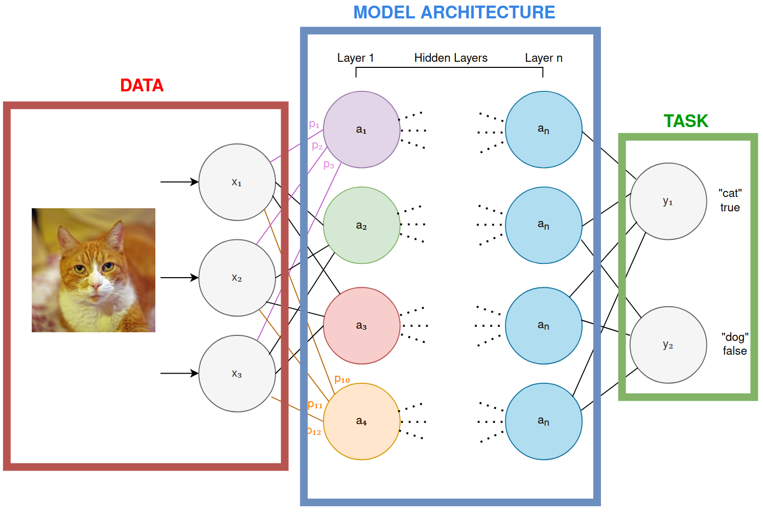
The ‘hidden layers’ that are shown in the deep learning diagram above have a magical property: through the mathematics of “nudging” parameters in the training loop, hidden layers and their neurons end up ‘specializing’ on smaller tasks within the overall task of predicting an output.
Let’s unpack that dense sentence with a diagram:
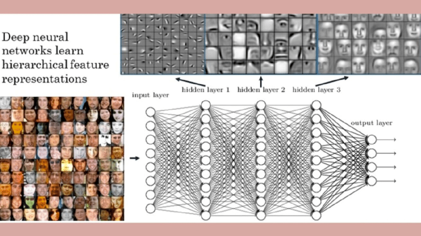
Here we’re trying to learn something about human faces (perhaps we’re trying to predict the mood of a face out of four different moods: happy, sad, neutral, angry). We feed the machine learning model lots of pictures of faces, and ask it to predict mood.
In order to perform that task, the model needs to learn skills that will help it better predict mood: what are the mouth and eyes doing, squinting? angled? etc. And in order to perform that overall task, the model will need smaller specialty skills, like finding edges in an image, finding contrast, identifying mouth, nose, eyes, and so on. If you look closely at the image above, you can see each hidden layer learning to perform those specialist tasks.
You can think of the “output layer” as asking the previous layer (the last hidden layer) for its judgment on the task that it’s a specialist in. That layer then asks the previous layer for its judgment, and then that layer asks the previous layer, and so on and so on.
This kind of implies that more layers means more specialties, allowing the model to perform more and more complex tasks. Too few layers, means the layers can’t break down problems into smaller tasks, and that may mean that output predictions are poor: just not enough collective expertise in the model.
This kind of intuition on how models are learning extends to even the most complex models, like Large Language Models (LLMs). You can imagine the last layer “I need to produce some text to respond to the input text I’ve been given” as that layer essentially asking all the previous layers (the experts) to work together to craft an appropriate answer. More on this point later, as the point is important to understanding how the intelligence of models will improve over time, surpassing human level intelligence.
Matrix Multiplication
The magic above of taking data and pushing it through many layers requires a massive amount of mathematical calculation. Computers are generally pretty good at calculating this kind of thing, but one piece of computer hardware is exceptionally good at it: graphics cards. The kind you would buy to run the latest and greatest games at the highest graphics settings. Getting from what a deep learning model looks like to running on a graphics card (GPU) is done through high school linear algebra and matrix math.
The following shows a simpler version of the neural network example above (without the activation functions), and shows how those calculations can be performed using matrix math:
 It’s not important to understand how this calculation works in detail, just that it can be represented and calculated using matrix multiplication.
This idea of using matrices to represent and calculate is important, as it explains why Graphics Processing Units are so excellent at building and training these big models: GPUs have been crunching matrix math for years. All those 3D games you play represent their visual scenes as polygons, the underlying representation being matrices! Rotating, flipping, clipping matrices is well known matrix math that has been optimized really well in the GPU hardware already – it’s great for deep learning.
What GPU hardware looks like and what it costs is detailed further down in the paper. For now, just think “deep learning equals matrix math which runs great on GPUs”.
What Deep Learning Models Look Like as Code
Let’s take a quick look at what machine learning models look like as software code. There is one dominant library/framework for using, building and researching machine learning models: PyTorch, which runs on the Python programming language. The distant second is Google’s TensorFlow. Google’s JAX (not displayed in the image below) is gaining ground as a fast neural network training framework.

The code below will show a PyTorch neural network model that will train and learn the XOR (eXclusive OR) truth table. The details of how the code is run isn’t important, as we’re just trying to visualize the structure/example of a neural network model:
| A | B | A XOR B |
|---|---|---|
| 0 | 0 | 0 |
| 0 | 1 | 1 |
| 1 | 0 | 1 |
| 1 | 1 | 0 |
import torch
import torch.nn as nn

class XOR(nn.Module):
    def __init__(self):
        super(XOR, self).__init__()
        self.input_layer = nn.Linear(2, 2)
        self.sigmoid = nn.Sigmoid()
        self.output_layer = nn.Linear(2, 1)

    def forward(self, input):
        x = self.input_layer(input)
        x = self.sigmoid(x)
        y = self.output_layer(x)
        return y
The code above is a PyTorch neural network model definition, with two input parameters, and one output.
xs = torch.Tensor(
    [[0., 0.],
     [0., 1.],
     [1., 0.],
     [1., 1.]]
)

y = torch.Tensor([0., 1., 1., 0.]).reshape(xs.shape[0], 1)
This code represents the training data that PyTorch will use to train the model above.
if __name__ == '__main__':

    epochs = 1000
    mseloss = nn.MSELoss()
    optimizer = torch.optim.Adam(xor.parameters(), lr=0.03)
    all_losses = []
    current_loss = 0
    plot_every = 50

    for epoch in range(epochs):
        # input training example and return the prediction
        yhat = xor.forward(xs)

        # calculate MSE loss
        loss = mseloss(yhat, y)

        # backpropogate through the loss gradiants
        loss.backward()

        # update model weights
        optimizer.step()

        # remove current gradients for next iteration
        optimizer.zero_grad()

        # append to loss
        current_loss += loss
        if epoch % plot_every == 0:
            all_losses.append(current_loss / plot_every)
            current_loss = 0

        # print progress
        if epoch % 500 == 0:
            print(f'Epoch: {epoch} completed')
The code above is the training loop.
# test input
input = torch.tensor([1., 1.])
print('XOR of [1, 1] is: {}'.format(xor(input).round()))
This code tests the model once it’s been trained. Running this code produces the following:
The result is XOR of [1, 1] is: 0
A more complex example that is both interesting, and reasonably trivial to train is having a neural network learn how to play the Nokia phone game “Snake”. This example uses a model architecture and training procedure called “reinforcement learning” – the training loop essentially plays millions of games of Snake, trying to learn the best strategies. The code for this can be found here.
Demo (after 10 minutes of training on a consumer grade GPU):
Size of Models and Time to Train
Training the XOR model is a trivial task, taking milliseconds. Training larger more complex model architectures can take months. Training time and training complexity is typically dependent on 1) how many parameters in the model need to be ’nudged’, 2) how much training data is required to have the model learn in a generalized repeatable way, 3) the model architecture used. There are more, but this is a high level rule of thumb. Some examples of training time, model size and compute required:
| Model | Training Time | Size | Compute |
|---|---|---|---|
| XOR | Milliseconds | 4 parameters | Laptop |
| Snake | Minutes | 12 parameters | Laptop |
| MNIST Digit Classification | Hours | 100-300 thousand | Laptop |
| ImageNet image classifier | 15-20 hours | 25-150 million | Desktop |
| YouTube Ranking and Recommendation | Weeks | Billions | Server Farm |
| ChatGPT 4 LLM | Months | Trillions | 10’s of thousands of GPUs |
| 2025 LLM Models | Months | 10’s of Trilliions | 100’s of thousands of GPUs |
| Future LLM Models | Months | 100’s of Trillions | Many datacenters |
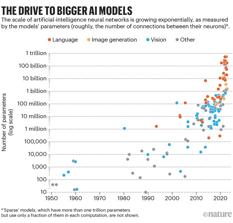
Nature has good graph that represents the exponential scale of AI model sizes:
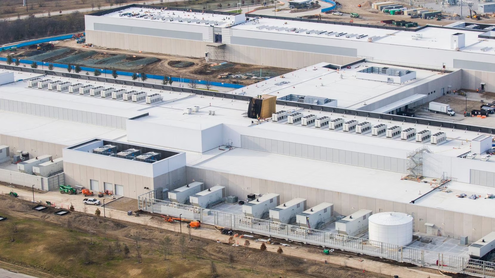
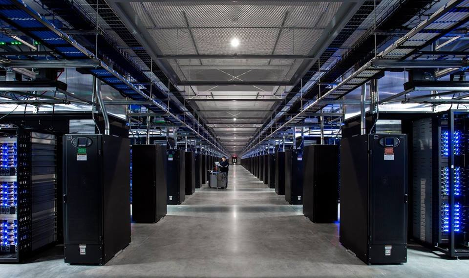
The compute required to train the largest and most complex models like ChatGPT is large and very expensive. The following pictures give a sense of scale:
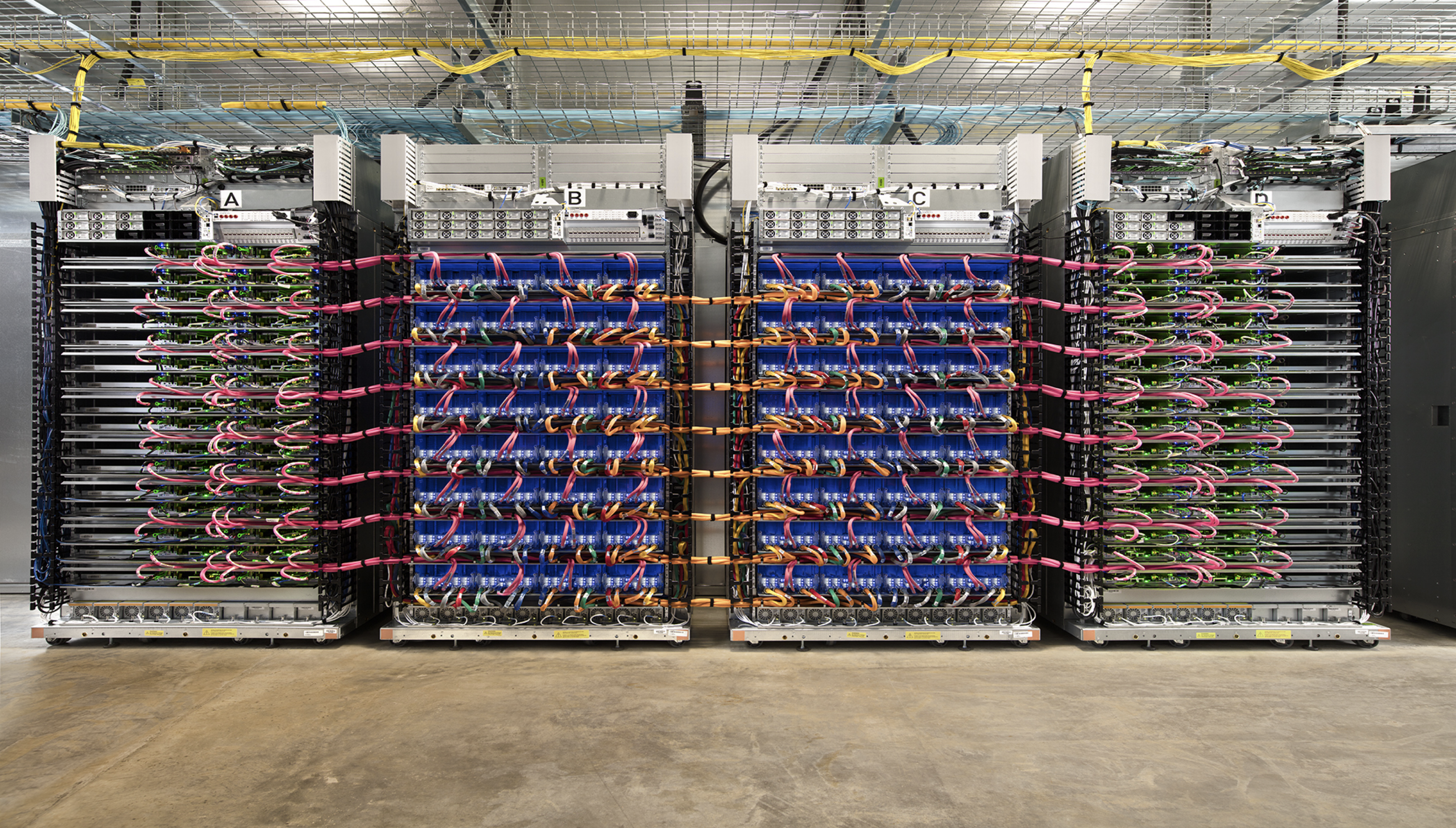
Facebook’s Fort Worth Data Center (2 full data center buildings):
Inside the data center:
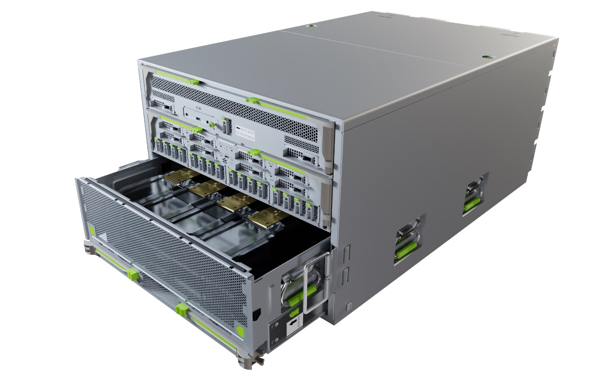
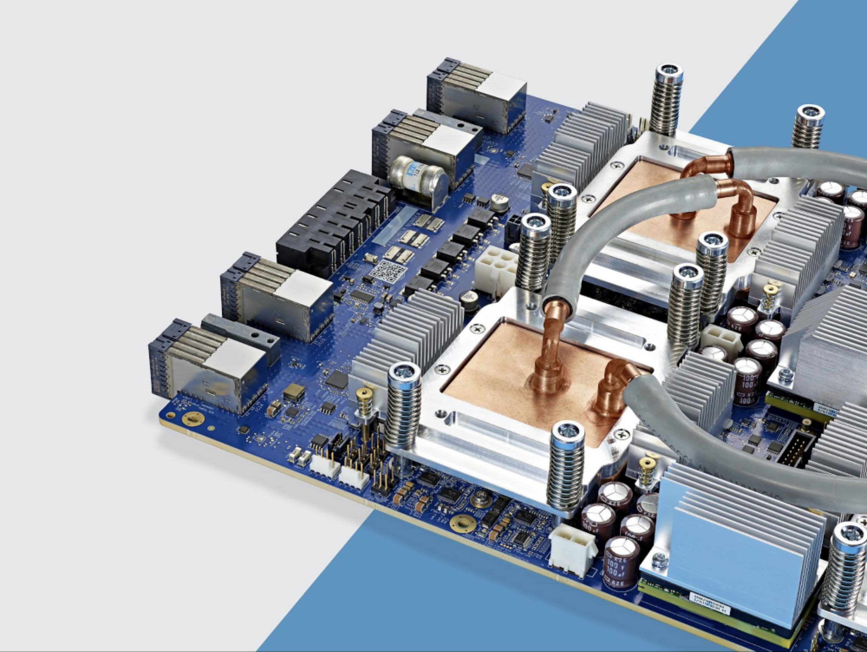
Rack based NVIDIA GPU Server, “Grand Teton” from Meta. Approximately 8x NVIDIA H100 GPU cards, ~15kw per rack typically:
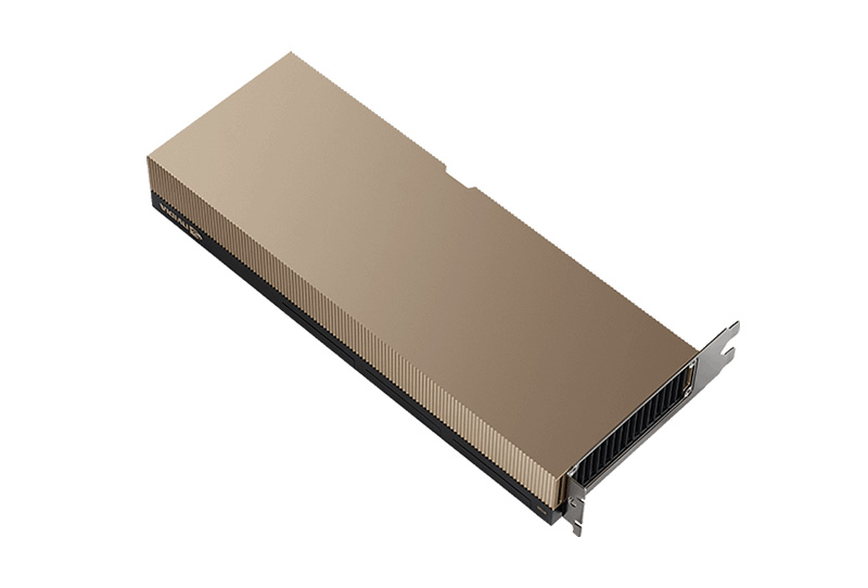
Single H100 NVIDIA GPU (Latest Generation 2023). ~800W power draw. Selling for ~$27k on eBay right now.
Exactly how many GPUs are required to train these latest super models like ChatGPT is an industry secret, but it’s understood that tens of thousands of GPUs were required for training over many months. Serving the finished model to the millions of customers that use it also requires 10’s of thousands of GPUs.
Google, Meta, Amazon and Microsoft have hundreds of thousands of GPUs available to machine learning researchers/practitioners to experiment on, build, and train models for production use. In 2025, it’s expected to have training clusters with 100’s of thousands of GPUs, and 2026+ will be millions.
Why so many GPUs?
Building and training a model that has trillions of parameters that need to be “nudged” requires that the underlying hardware have a) enough memory to hold the parameters that are being nudged while training, and b) enough computation power to perform the matrix multiplications and nudge the parameters to reduce error in a reasonable time on human scale (months, not years).
Trillions of parameters requires a lot of memory:
- 1 trillion parameters = $1 \times 10^{12}$, assuming each parameter is a 32 bit floating point number, then each parameter is $4 : \text{bytes}$.
- Memory required to hold all the parameters: $1 \times 10^{12} \times 2 \times 4 : \text{bytes} = 8 : \text{TB}$
- You also need space to hold the results of the matrix calculations, book keeping and more, so roughly we end up with ~ $20 : \text{TB}$ of memory required.
- This implies you need at least 256 H100 GPUs that have 80 GB of memory.
Why is it that models need tens of thousands of GPUs?
Big models require big compute:
We want to speed up the training and nudging of the parameters. More GPUs means faster nudging. GPUs and other AI hardware usually measure how fast they are by stating how many floating-point operations per second they can achieve (or how many of those matrix calculations they can perform per second to do the nudging). There are many different “precisions” of floating point numbers - in general, the more precise, the slower the operation - which means there are many reported “FLOPS” (floating point operations per second) numbers depending on the precision you want. We’ll focus on the common one for LLM training: BFLOAT16 (sometimes called “brain float”) which is 16 bits (or 2 bytes) of precision.
The current H100 GPU from NVIDIA can do 2000 terraFLOPS (or 2 petaFLOPS) of BFLOAT16 calculations. The previous generation NVIDIA A100 could do 624 terraFLOPS. H100 is a clear step up in terms of computation. Tens of thousands of GPUs means a huge amount of BFLOAT16 compute: 2 petaFLOPS times 10,000 is:
$$ \begin{align*} 2 : \text{petaFLOPS} &= 2 \times 10^{15} : \text{FLOPS} \newline 10{,}000 \times 2 : \text{petaFLOPS} &= 10{,}000 \times 2 \times 10^{15} : \text{FLOPS} \newline &= 20{,}000 \times 10^{15} : \text{FLOPS} \newline &= 2 \times 10^{4} \times 10^{15} : \text{FLOPS} \newline &= 2 \times 10^{19} : \text{FLOPS} \end{align*} $$ This means 10k H100 GPUs are roughly capable of $2 \times 10^{19}$ floating point operations per second. (In practice, they can’t actually achieve that much because of a lot of overheads we won’t get in to here).
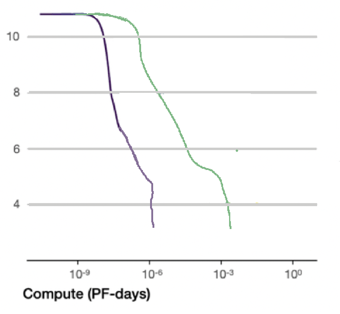
The following graph from epochai.org shows how many floating point operations (or parameter nudges) were required to train various released models to have the smallest amount of error:
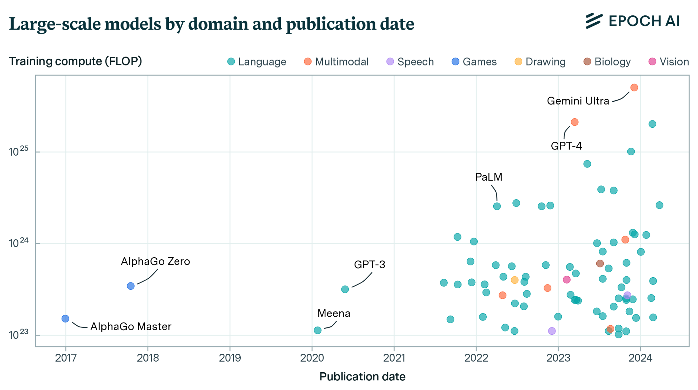
If ChatGPT 4 required roughly $5 \times 10^{25}$ floating point calculations, we can roughly determine how long the training time would be by dividing the amount of FLOPS needed to nudge the parameters, by the amount of GPU FLOPS hardware compute we have available ($2 \times 10^{19} : \text{FLOPS}$). The more GPUs we have, the less time it takes to train:
$$ \begin{align*} Time = \text{Total compute needed} \div \text{Compute capacity per second} \newline Time = (5 \times 10^{25}\ \text{FLOPS}) \div (2 \times 10^{19}\ \text{FLOPS} / sec) \newline Time = 2.5 \times 10^{6}\ \text{seconds} \newline Time = 29\ \text{days} \end{align*} $$ GPUs almost never reach peak FLOPS performance while training: communication overhead between host and GPU, or intra-server comms overhead, or other bottlenecks, typically means you get ~20-30% efficiency. This means a GPT 4 sized model will take approximately 100-150 days or so to train on a cluster of ~10,000 H100s.
More GPUs Means More Degrees of Freedom
In general, more FLOPS and more memory means more degrees of freedom in model size, model architecture, and how long the model will take to train. It also means:
- Researchers can explore bigger and more complex model architectures to achieve learning of more complex tasks.
- Higher velocity of output of research and model experimentation: faster training equals more experiments
- Global scale deployment of complex machine learning models for your customers/users.
And most importantly, more GPUs means more intelligence, as we’ll now explore:
Scale and Intelligence of Large Language Models
The largest models on the graph above are all LLMs and its worth taking a special sidebar to understand why. A deeper “what are LLMs” tour is further down the document. First, a few things worth noting before talking about scale and intelligence:
- While ChatGPT, Claude.ai and so on are called LLMs, you can now say they’re just “large models” as they go beyond reading and writing natural language to ingesting and generating images, speech, and soon video.
- LLMs aren’t just Q&A “chatbots”. While ChatGPT popularized this form of LLM interaction, there are vast ways of using these models. One popular form is calling the model via software through an API, where software can instruct the model to generate code, perform computation, interpret and rewrite text and images and so on. Through this lens, the LLMs act as sort of a “computer” - instead of programming the computer via code, you’re programming the computer via natural language instruction.
- Most of the frontier power of these models currently comes through “programming” them through very sophisticated techniques; techniques often not available to users through the web or mobile application.
GPT 4 had roughly $5 \times 10^{25}\ \text{FLOPS}$ of training compute pushed into a model size of 1.8 trillion parameters, using a rumored ~25k A100 GPUs. The cost at the time of these GPUs was roughly ~$25 thousand USD per GPU to purchase, ~$625 million USD in capex. GPT 4 used ~300 times more compute to train, does that mean its 300 times smarter? No, but “it’s complicated”.
Scaling Laws
The rush for FAANGS and others to purchase billions of dollars in compute for training LLMs can be traced and rooted to the seminal paper Scaling Laws for Neural Language Models which was written by OpenAI researchers (five authors on that paper have left OpenAI and started Anthropic, another LLM frontier model company).
The papers core contribution is the finding that as the number of parameters in an LLM increases, its performance tends to improve following a power law relationship (y-axis is “error” of the model) (not to scale of the actual scaling laws):
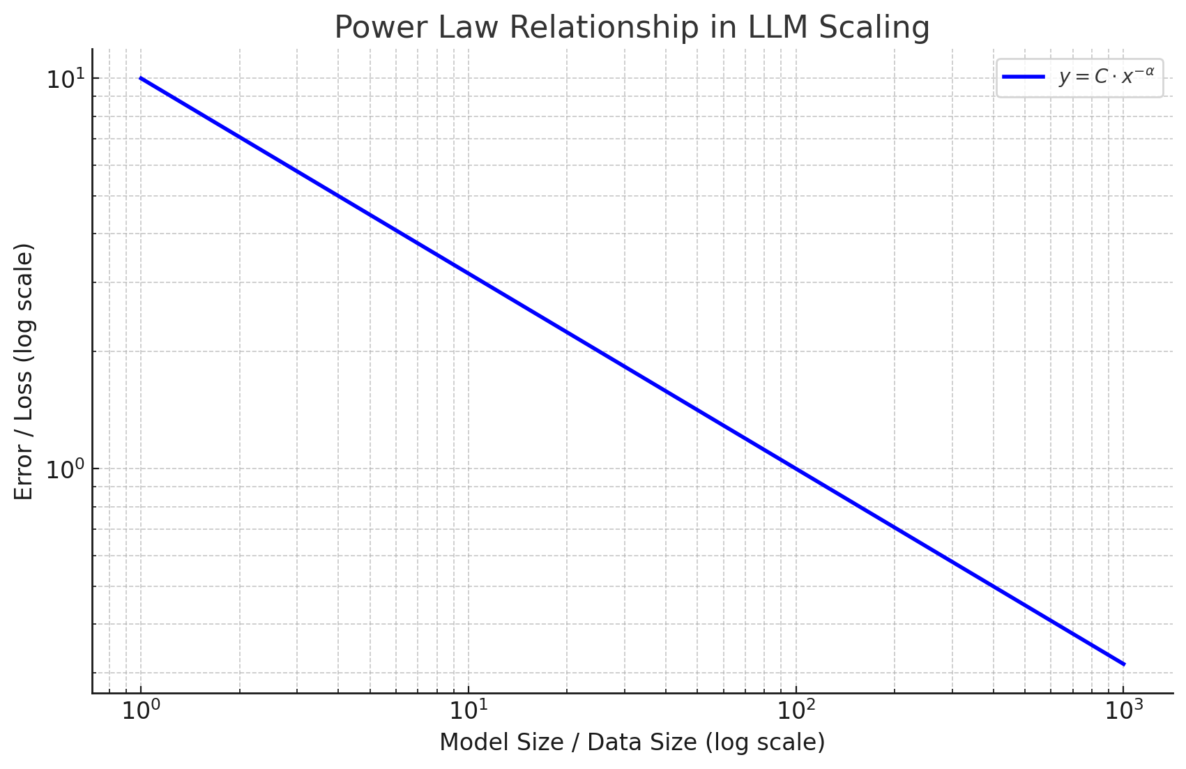
The paper also describes the relationship between compute, amount of data, model architecture, model size and the “error” of the model. This means for a given input, let’s say “data size”, you can calculate the most optimal model size, compute and training time for that input. Or given FLOPs you have available, you can calculate how much data you need, the model size, training time and so on. Unfortunately, it doesn’t provide a precise calculation of the intelligence of the model, as this tends to be non-proportional to compute and difficult to predict.
In practice, model capabilities tend to improve in unpredictable “step changes”, or simply “emerge” at a given compute factor. It’s thought that these step changes come out of improvements in foundational intelligence: reasoning ability, understanding context better, broader knowledge and so on - higher order skills start to “click”, much as they do in humans when they age. Some skills may also plateau for some time before taking off again, which makes predictions of model size to skill difficult. Scaling laws provide “potential for improvement” not a guarantee.
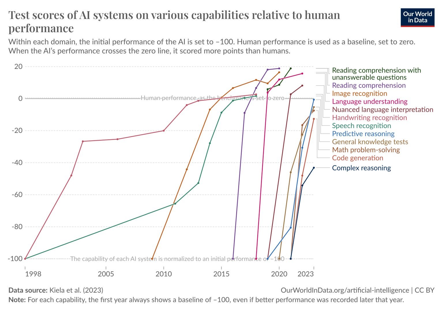
The paper shows several graphs illustrating the effect of compute and size, with respect to loss (error) over different domains:

Given the focus on scaling in the past few years by researchers, and the huge capex investments made, we’re seeing clear improvements in model intelligence (0 on the y-axis is benchmark human performance on the given task):
Large US tech companies are rushing to capture and deploy the supply chain of deep learning training compute to try and train AGI first:
| Company | 2024 YE (H100 equivalent) | 2025 (GB200) | 2025YE (H100 equivalent) |
|---|---|---|---|
| MSFT | 750k-900k | 800k-1m | 2.5m-3.1m |
| GOOG | 1m-1.5m | 400k | 3.5m-4.2m |
| META | 550k-650k | 650k-800k | 1.9m-2.5m |
| AMZN | 250k-400k | 360k | 1.3m-1.6m |
| XAI | ~100k | 200k-400k | 550k-1m |
Estimates of GPU or Equivalent Resources of Large AI Players - lesswrong.com
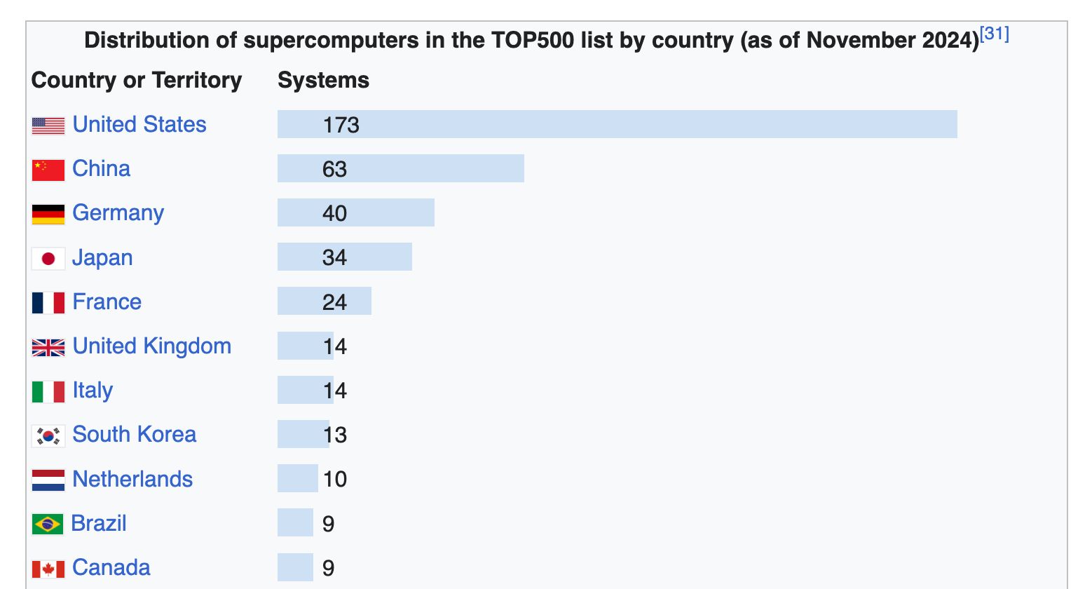
The US and China dominate the TOP 500 list of supercomputers:
Given the cost of these FLOPs, and more FLOPs meaning larger and more intelligence models, there’s a race to bring the $\frac{\text{cost}}{\text{FLOPs}}$ cost per flop down by creating cheaper and more efficient hardware.
It’s worth taking a sidebar to explore this race to reduce cost and speed up deployment, as it has various strategic consequences for the industry, and for government sovereignty:
Training and Serving Costs and Constraints
Optimization and cost savings for training and deploying machine learning models (in particular, LLM models) has become critical. In general, FAANG’s, large enterprise, and cloud providers are optimizing for the following things:
- Performance per Dollar: floating point operations per second given capital and operational expenditure costs of hardware.
- Performance per Watt: floating point operations per energy usage. Power is now a dominant planning constraint for datacenter build outs.
- Machine Learning Researcher experiments per unit of time: more experiments mean more insights and model improvements.
- Data collection and preparation.
Optimizing (1) and (2) above can be achieved in numerous ways:
- Hardware vendor choice
- Hardware vendor software stack
- Limiting/refining/curating training data (thus reducing how long training takes)
- Trading off model accuracy for reduced training time
- Model architecture improvements (decreasing parameter count, alternative choices in model architecture, etc)
- Compressing models (a technique called quantization, which trades off model accuracy by shrinking parameter size)
- Reducing “freshness” of the model (reducing how often you re-train the model)
- Using “off the shelf” models instead of training your own.
Creating a strategy for reducing costs and unblocking constraints is more art than science right now, as (1) through (8) are often difficult to measure, and difficult to connect to product/customer impact.
Costs to train and deploy will differ depending on:
- The complexity of the model being trained/deployed
- How many end-users are using the model in production
- How often the model needs re-training
- From scratch training, or fine-tuning/extension from existing model (see below).
The “Size of models and time to train” section above gives a general sense of training compute requirements. Deployment (or “inference”) requirements can vary and depends almost entirely on the size of the customer base that will use the model at any given point in time.
LLM Costs and Constraints
Scaling laws indicate that the path to increasingly capable AI systems, potentially including AGI, is largely a matter of training and serving for size. This requires overcoming four key constraints: the silicon supply chain, power infrastructure, networking capabilities, and the velocity of datacenter construction.
This paper reverse engineers the requirements for training a 100 trillion parameter “AGI like” LLM model, which helps us understand the magnitude of these constraints:
-
Silicon Supply Chain and Silicon Cost: Approximately 1.6 million GPUs with ~313 petabytes of HBM memory will be needed. This represents an unprecedented demand on semiconductor manufacturing, requiring significant expansion of current production capabilities. At current market prices (~30k USD per GPU), the hardware alone would cost ~48 billion USD, excluding networking and infrastructure costs. Recent announcements like Microsoft and OpenAI’s $100 billion data-center project reflect the scale of investment required.
-
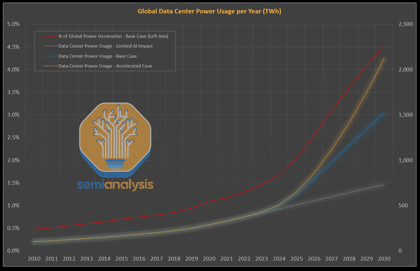
Power Infrastructure: ~3 gigawatts of power for GPUs alone, scaling to ~4-5 gigawatts total to house in datacenters. This far exceeds current datacenter norms, where most facilities built in the past ~5 years use 50-300 megawatts. Even Australia’s largest proposed datacenter, NextDC’s S4 Sydney, caps at 300 megawatts. This SemiAnalysis graph shows the projected global datacenter power usage under different AI acceleration scenarios, illustrating the magnitude of power required, measured in multiple percentage points of all US energy capacity:
-
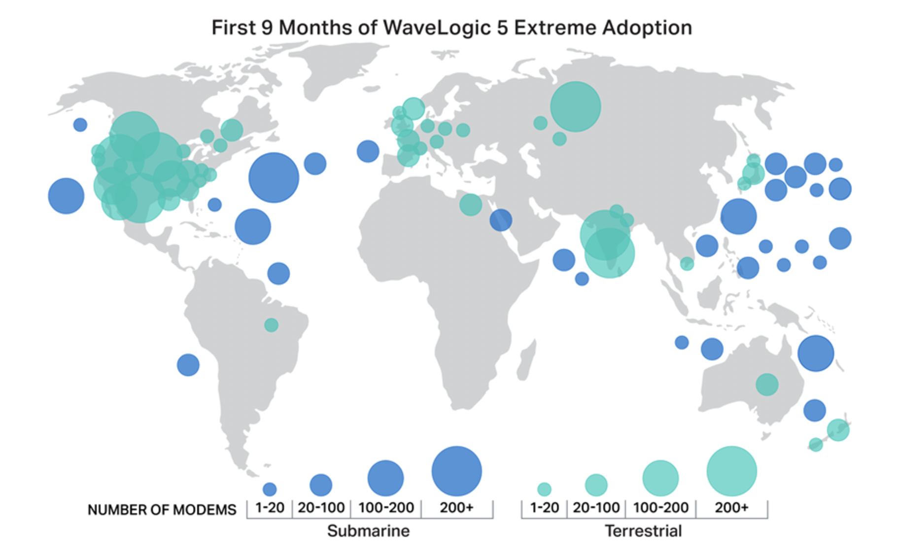
Networking: Training at this scale requires multiple datacenters connected by extremely high bandwidth networks. Training is high demand, highly data distributed, meaning low-latency, and extremely high bandwidth intra-datacenter connectivity is required to ensure intra-datacenter communication does not become a training bottleneck. 400Gb/sec - 800Gb/sec intra-datacenter links are relatively common in the US and China. Multi-terrabit fiber is being rolled out also. Hard to see the trend here, however, unsurprisingly the US is ahead on rollout:
-
Datacenter Construction Velocity: The pace of datacenter construction must accelerate to accommodate current training demand. Current construction timelines are a bottleneck for AGI players. Meta’s Q2 2024 earnings already signal this trend with significant increases in capex spend to speed-run datacenter construction.
Currently, the US and China are dominating the race to invest in infrastructure to unblock these constraints. The UK Government has recently announced its AI Opportunities Action Plan to try and catch up, along with roughly 14 billion pound worth of data center projects and a new supercomputer.
Given silicon supply and power consumption are the two dominant factors in training and serving LLMs, there are several efforts to build new machine learning accelerator chips with a focus on reducing power consumption, and decreasing cost/FLOP. These potentially have the ability to unseat NVIDIA as the dominant hardware provider (along with beating down NVDIA’s 70% margin on chips).
Machine Learning “Accelerator” Hardware
You may have heard about specialized hardware that hyperscalers like Google and Amazon have built, an example being Google’s “TPU”, and Amazon’s Trainium. This hardware looks and acts very similarly to GPUs, but may have a different configuration (compute, available RAM, connectivity to other TPUs etc) that may be more specialized to a particular type of model.
Here’s a picture of an older generation TPU (the plastic piping is used for water cooling), and another picture of many TPUs connected together in a data center rack:
Specialization is always in the interest of optimizing cost, power and performance for a particular set of workloads. GPUs in themselves are a form of specialization originally for computer gaming: GPUs are great and drawing and manipulating triangles, significantly better at it than the original Intel x86 processors. As mentioned in this doc, that game engine specialization tends to be helpful for AI training also. GPUs however, also have a bunch of silicon dedicated to game engine tasks that are not at all related to neural network parameter nudging.
AI Accelerators like TPUs and Trainium have more silicon dedicated to the act of AI training and inference, and spend more silicon on accelerating the critical path of training and inference. For instance, on-chip silicon is dedicated to extremely fast intra-chip communication, so that the neural network can be distributed across many chips to cooperatively work on nudging parameters of the entire model in parallel.
Extracting the full performance out of these accelerators is done via a software layer, sometimes called the “deep learning compiler” or “neural network compiler”. This software takes the architecture of the model that is described by humans (amount of parameters, layers and so on), and generates code that the chip can understand and execute in order to perform the training and inference operations. This sounds simple, but it’s actually incredibly complex to get right: you need the software to figure out the exact right code and layout that will be “mechanically sympathetic” to the hardware, so that you push the hardware hard in the places it excels, and avoid asking too much of the less efficient parts. It’s possible to have 2x faster and more efficient hardware, but the software compiler generate unsympathetic code that ends up running 2x slower.
Compute Efficiencies (or CE’s)
Specialization of machine learning hardware is considered to be a “compute efficiency”, which is a term given to an improvement in any part of the stack which gives you the same amount of loss, for less compute. A “2x” CE (compute efficiency) largely means it requires 2x less FLOPs to get the same error loss.
This is what a loss curve would look like, comparing one model training run with a 2x CE, vs. not:
Compute Efficiencies come from all places in the AI stack: data (mixture, ratios etc), hardware (choice of hardware), architecture of the model and how sympathetic is is to the hardware, writing custom kernels (CUDA kernels for instance) to make training/inference faster, quantization, model distillation and more. The size of a given model is correlated to intelligence, but a smaller model with more compute efficiencies can be higher performing than a larger model without.
For frontier LLM companies in particular, these can be worth 100’s of millions of dollars, and are considered company secrets. You can spend your CE by making a smart model cheaper, or making a model much smarter.
A Deeper Look Inside an LLM Model
Large Language Models (LLMs) deserve its own “what is” section, as there are multiple properties of LLMs that are unique and which will likely drive more non-linear value generation than any other model. The most commonly used LLMs right now are OpenAI’s ChatGPT, Anthropic’s Claude Google’s Gemini, and the Open Weight model Llama from Facebook.
The most common way LLMs are used today are:
- User/Assistant conversational chat-bot where users ask questions and ChatGPT generates answers.
- Education: Information retrieval and synthesis, conversational style “explain to me how this works; I don’t understand this…”.
- Generative/Creative: “generate me a limerick that talks about my Australian friend who likes Pinball”, or “generate me Python code that calculates compound interest”.
However, ChatGPT (and other large language models) have non-obvious abilities which make them powerful reasoning, prediction and probabilistic cognition engines that happen to be both introspective and programmable. And that programming (through prompt engineering) takes place at an abstraction level that is available and accessible to everyone. These non-obvious abilities puts them directly in competition with flesh-and-blood cognition engines, and their eventual wide distribution and ease of specialization through natural language programmability means they will eventually get inside every workflow, every prediction and every decision.
Reasoning and Decision Making through LLM Programming
Let’s take a look at an example of these non-obvious abilities, starting with reasoning and decision making. Imagine I would like help with sourcing engineering candidates for my imaginary “silicon engineering” job. This job requires specialization in building emulation environments for an ASIC (custom silicon). I’d like to source candidates that closely match my job requirements, and I’d like to also find candidates that overlap substantially but could be trained in the particular ASIC specialization.
Prompt, or the “programming”:
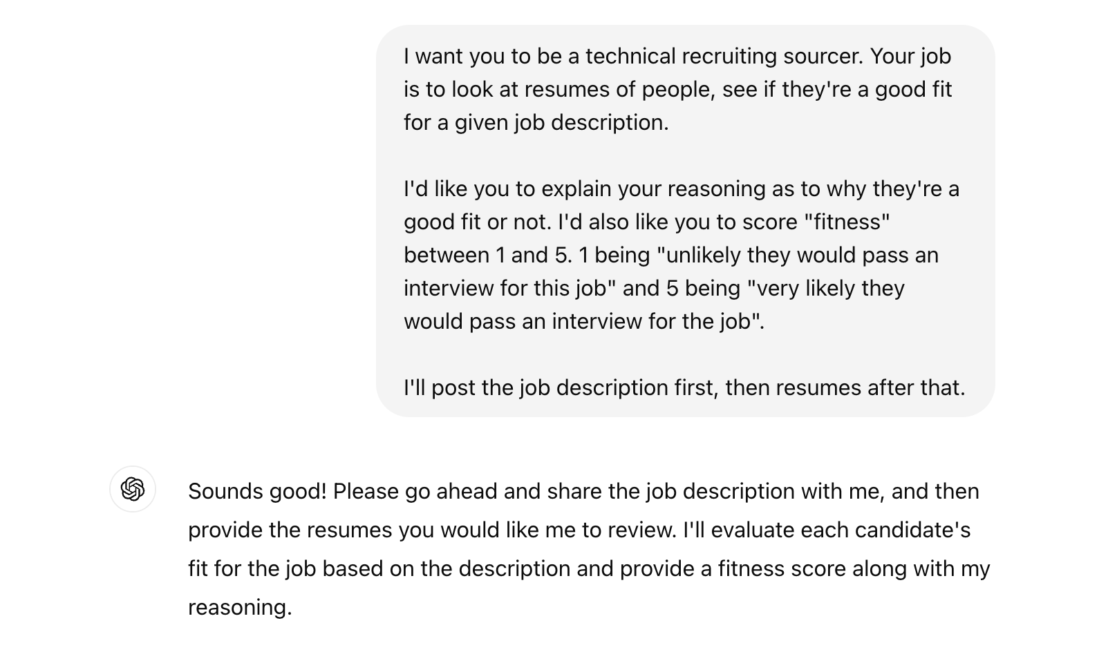
The job description:
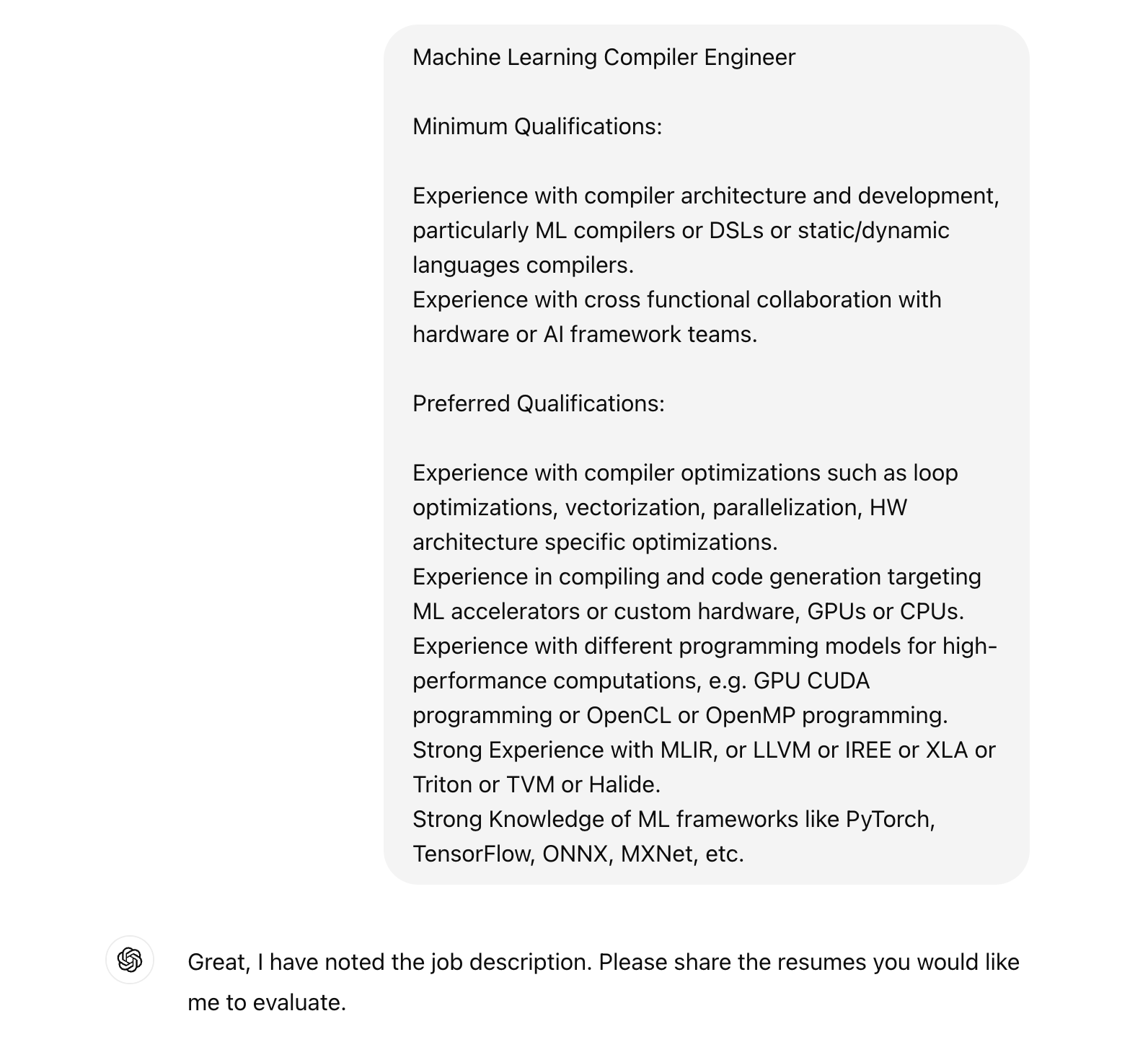
The candidates resume and result:
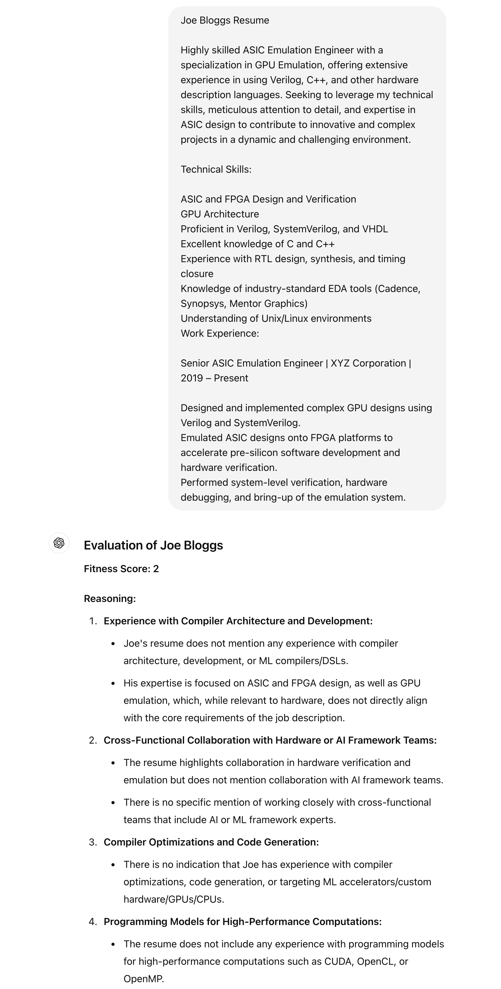
ChatGPT 4o ends up summarizing:
Fitness Score: 2. While Joe Bloggs has a strong background in ASIC and FPGA design and GPU architecture, his experience does not align closely with the requirements for a Machine Learning Compiler Engineer. The lack of relevant experience in compiler development, ML frameworks, and high-performance computing programming models results in a low fitness score for this specific position.
ChatGPT 4o was able to compare and contrast resume to job description, and understood that some of the candidates missing job requirements were more or less relevant than others. It performed this reasoning with a level of sophistication approaching a reasonable technical sourcer (and far exceeds sourcer/recruiter tooling that tend to perform basic string matching between resume and job description).
Let’s try a more sophisticated example, where we’re asking ChatGPT to behave like it is a “virtual computer”, one which executes a set of instructions. This kind of programming requires that the model have an exceptional reasoning and instruction following engine to ensure that it correctly interprets the initial “programming prompt” and the subsequent programs.
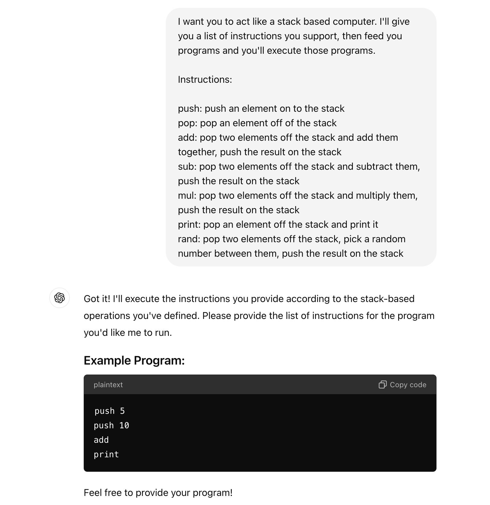
Let’s give it a program:
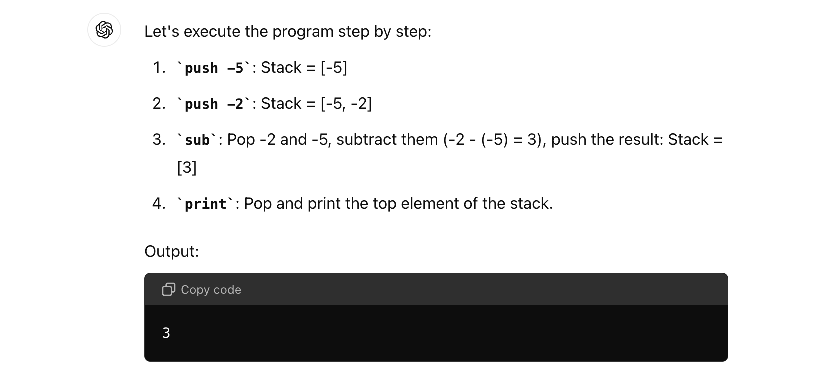
It defaults to -2 and then -5 as the order of the “sub” operation, giving us -2 - -5 = 3. Reasonable, given -2 was on the top of the stack. But this ordering convention is arbitrary, and perhaps I wanted the reverse convention instead?
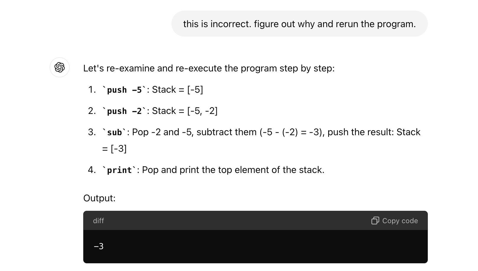
GPT4o reflects on the conversation, figures out the error (ordering must be the error) and reruns the program with the corrected result.
Above is an example of introspection, abstract reasoning, decision making and creating a “mental simulation” of a user described world - one which young humans might struggle with. A valid question to ask is “is this just a recreation of the training data?”, after all, stack based virtual machines are a common thing in computer science. Fields of study have spun up around this question, most prominently “interpretability”, and while still early, evidence seems to suggest that LLMs are going far beyond “parroting” training data, combining skills in ways that it had not seen during training. Other papers (1), (2), (3) have similar conclusions.
How do LLMs Work?
Stephen Wolfram does an exceptional job of explaining the “under the hood” details of how LLMs are trained, and how these LLMs end up producing magical and almost human like output. It’s impossible to succinctly summarize this explanation, so instead I’ll give a very high level set of abstractions and analogies:
- LLMs take text as input, and as output, try and predict what the best text might be to “complete the rest of the text”. Thinking about this in terms of the chatbot model, the input text is the question, the answer is the output text.
- It learns how to do this by looking at trillions examples of sentences, paragraphs, natural language and images from the Internet.
- It figures out interesting and non-obvious statistical associations between words and a collection of words in sentences, and builds probabilistic models from them. These associations are used to generate the output text.
- If you remember back to the example of “specialization” that occurs in hidden layers when training a neural network to detect faces (see image below), the same thing is happening in these LLM models. You can abstractly think about it as the output layer asking all the layers before it “hey, I need to generate text to answer the users question, I need all you experts to help put together an answer for me”. These massive models are forced to learn millions of specializations and expertise in “generating limericks”, or “produce facts about the civil war”, and so on.
- These experts aren’t just limited to understanding and generating natural language – LLMs can read and produce computer code, math, spreadsheets, images, video and more.
The LLM Roadmap
Quite a few of the trends were identified in previous sections, so let’s recap them before exploring the potential LLM roadmap in more detail:
- Current generation models (GPT 4, Gemini, Claude 3) cost roughly 100’s of millions in capex and opex to train and deploy, with $5 \times 10^{25} : \text{FLOPs}$ worth of compute in them.
- Estimated 20-40 thousand GPUs required for training GPT4 and therefore ~$500+ million USD in hardware expenditure. Gemini likely used TPU accelerators for training which would have a different cost/FLOP calculus.
- Estimated 13 trillion tokens of data was used for GPT4.
- All frontier LLM models are multi-modal with at least image and text as input, some with speech, and image, text, speech outputs.
- LLMs during training end up with “millions of specializations” embedded in their parameters. More parameters and compute usually means more and better specializations.
- GPT, Claude and Gemini largest frontier models with roughly trillions of parameters. Meta has their “open weight” model Llama, a dense model with 405b parameters.
- Model access via chat interface, or via API access.
- Emphasis on scaling intelligence through Post-Training: reinforcement learning and “test time compute” (more on this later).
A good and recent interview with Dario and Daniela Amodei from Anthropic foreshadows what to expect in terms of size and cost for models: ~$100 billion USD. Implied in this view is that LLM Scaling Laws continue to avoid s-curve diminishing returns, and continue to produce value and return that exceeds the cost. The “LLM Training Costs and Constraints” section briefly reviewed a paper describing the requirements for a 100 trillion parameter model, costing roughly $50 billion. To recap:
- 15 petabytes of data tokens
- ~1.6 million GPUs with ~313 petabytes of HBM memory
- ~3 gigawatts of power for GPUs alone, ~4-5 gigawatts for the datacenter
To understand what will these $100 billion dollar models will look like, let’s take a quick look at the way they’re used today and the current limitations. Today, when using an LLM, you’ll find the following:
-
A chatbot style request response paradigm: A user has a question or problem, and works through that with the LLM like a human converses with another: provide some context, ask the question, get an answer, clarify and explore the answer:
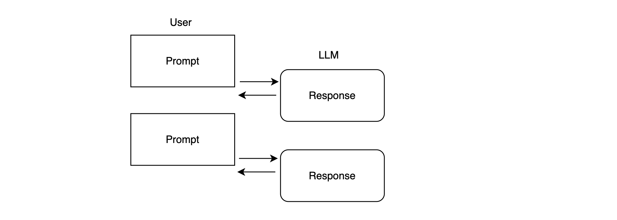
-
A limited context window or “memory” for the LLM: most LLMs have limited memory you can work with, roughly between 100,000 and 200,000 tokens (although Gemini has a million token context window). This is the upper limit on the amount of information you can tell the LLM before it stops you from sending more - 50k tokens is roughly the size of the book “A Brave New World” by Adlous Huxley. You can essentially “teach” the LLM four books before asking the question you want to ask.
-
While LLMs have been trained on all the tokens on the Internet, the act of training means that the data on the Internet is kind of “filtered and compressed”. Things that are really important will be learnt by the training process with nuance, and things that aren’t important will be compressed and summarized into the parameters of the model. Asking an LLM about the Prime Ministers of Australia, the LLM will have a nuanced understanding and be able to respond in kind. A random persons blog on the Internet, the LLM may have either filtered or compressed that information into a very high level summary.
-
Data the LLM hasn’t seen (e.g. data in your enterprise about your customers or something) needs to be fed to the LLM for it to be reasoned about: there’s simply no way it would have been trained on that data as its behind your firewall.
-
LLM models don’t currently integrate new data and knowledge into their parameters (i.e. they’re not continuously training). They don’t benefit from influencing and being involved in reinforcing feedback loops.
The above means that in order for an LLM to reason about things within your firewall, you need to collect up and send the LLM that data first, before having the LLM do things for you. With only four books of context memory, this means that you can’t give the LLM your entire enterprises data for each request - you need to be selective, and package the data most relevant to the query. There are systems that automate this task (Vector Databases, Retrieval Augmented Generation or RAG, and so on) but efficacy varies.
Next generation models will lift these constraints:
- Request/response chatbot paradigm will evolve to be reactive, agentic and independent (more on this below).
- Models will have unlimited or near unlimited context windows, or the ability to “upload your data” for the LLM to have pre-computed understanding of that data.
- Models will be “continuously” training and participating in feedback loops by virtue of having unlimited context windows.
Reactive Agentic LLMs
LLMs will go beyond current User -> LLM request and response chatbot style interaction paradigms to be independent “always running” agents that can do the following:
- Work on long running tasks: first minutes, then hours, days and weeks long.
- Work cooperatively with other agents that are also running independently - enabling the breakdown of large tasks in to smaller tasks which are then distributed to workers to work on in parallel.
- React to environmental changes instantaneously: e.g. an agent that is constantly reading and reacting to news to place trades on a stock market.
- Perform experimentation and simulation to discover new and novel things.
Tasks right now, particularly in the chatbot “request response” paradigm, are minutes long. Future releases will be able to perform long running computation:
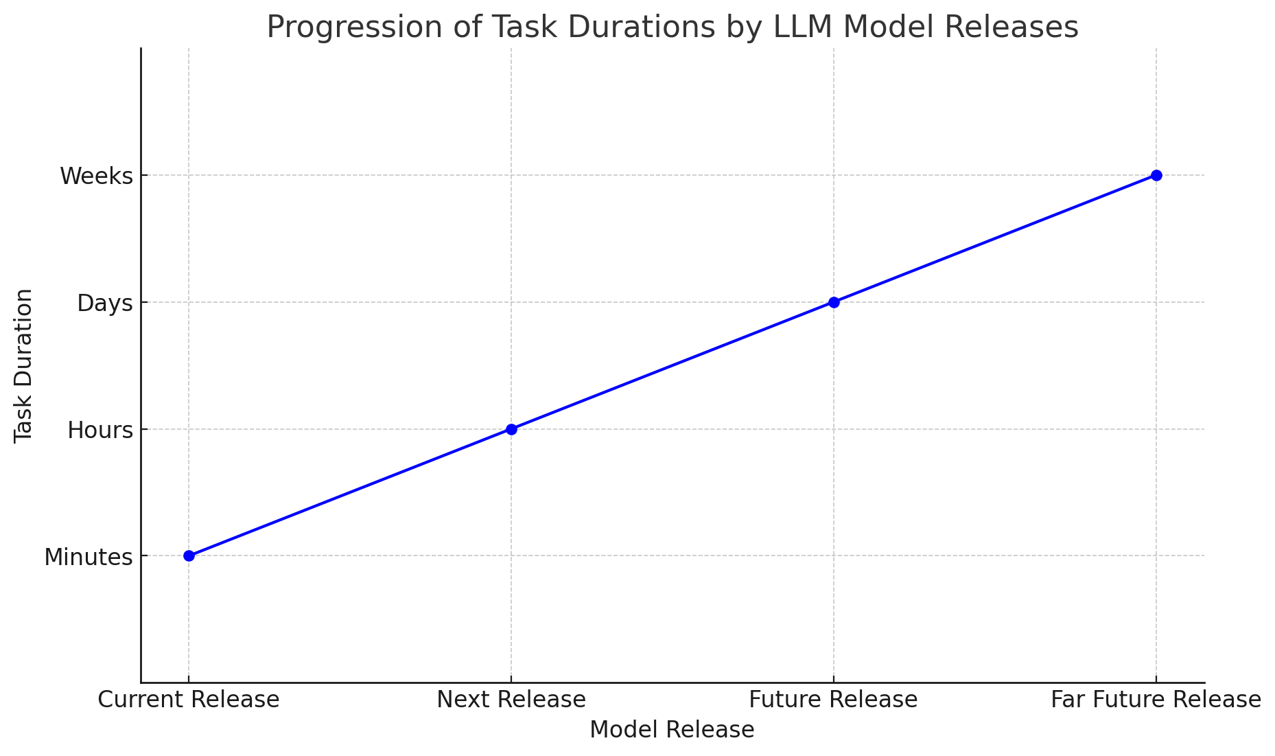
Both task sophistication and duration will go up, and amount of cooperative compute (i.e. many agents working on sub-problems) also goes up. This is strongly correlated to model intelligence, mostly due to a) how well the LLM is connected to the outside world, and b) how effective it is at breaking down problems and correctly and successfully completing those problems. And (b) is particularly important: usually most steps of problem solving need to be correct as they are inputs in to the next step of the larger problem.
LLMs can do this in the small form today by generating code to helper tools that can be executed on a computer. Let’s look at an example task:
go to https://ten13.vc/team and get the names of the people that work there
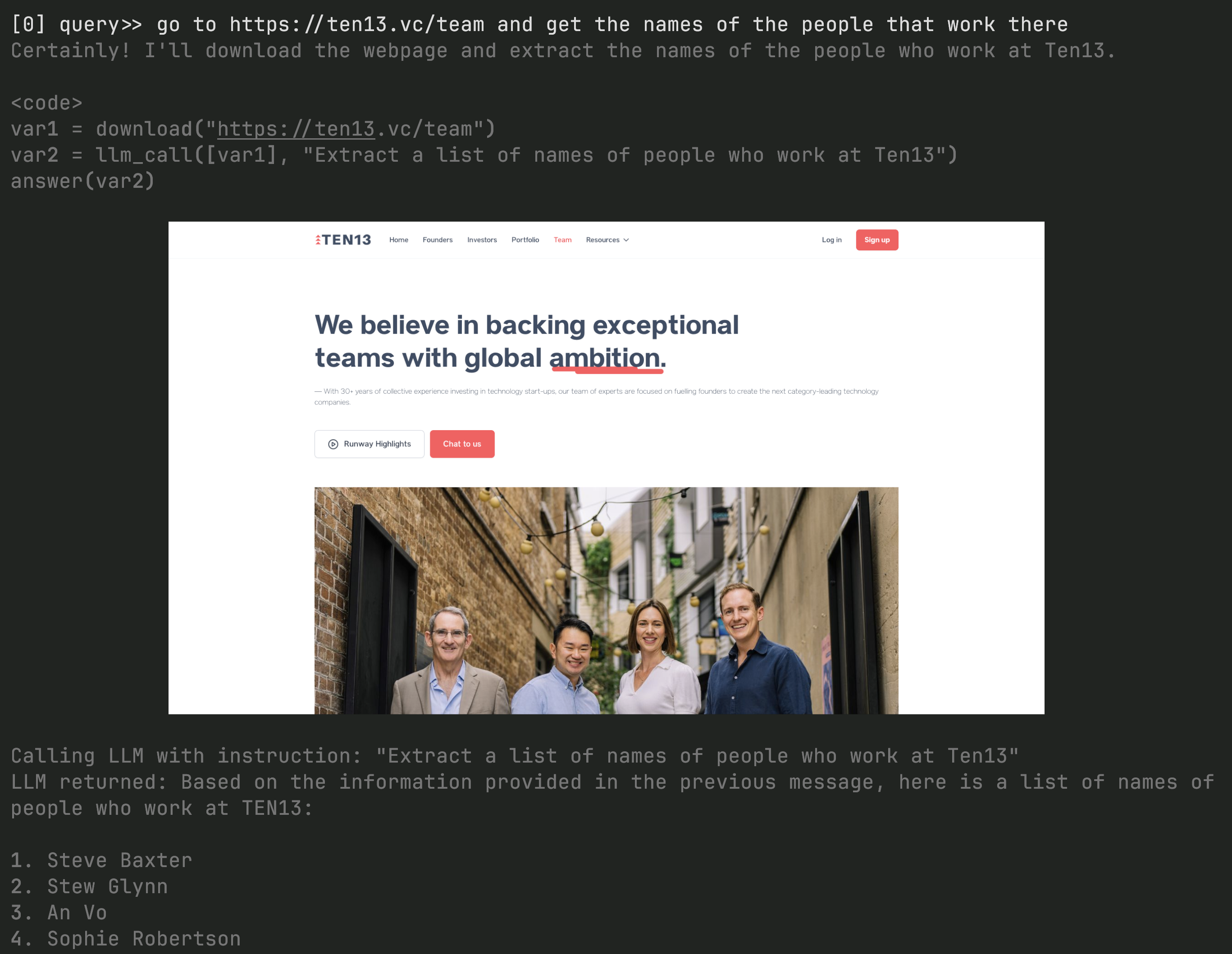
The white colored text is the query, the grey colored text is the LLM responding to the query. It has generated the following code:
var1 = download("https://ten13.vc/team")
var2 = llm_call([var1], "Extract a list of names of people who work at Ten13")
answer(var2)
The two helper tools that the LLM is using are download and llm_call. The download helper uses a web browser to connect to the web page on behalf of the LLM and downloads the page. The llm_call helper tool packages up the webpage and sends it back to the LLM for processing.
This interleaving of LLM describing the breakdown of problems via natural language, and then generating code to solve them works quite well right now given how well the current generation of models generate computer code. However, task complexity and duration can be a problem because of a few constraints:
- The code generated can be incorrect
- The semantics of the code are incorrect: i.e. it’s misunderstood the task but generates correct code
- The data that the code is working with is too large to fit in to the context window of any subsequent LLM calls: i.e. the webpage that is downloaded is larger than the LLM token limit.
The analogous situation is a junior programmer compared to a senior programmer - complex tasks are more difficult for a junior programmer to get right. The more tasks there are to solve, the more likely the whole task is going to be incorrect.
With model intelligence going up with each model generation, and larger (and perhaps unlimited) context windows coming, these constraints loosen, leading to more complex and longer running tasks having a higher probability of success.
Unlimited Context
Context windows (or token size constraints) are a constraint driven by underlying hardware constraints and LLM architecture choices. Performance of the model (i.e. how many tokens per second the LLM can process) are also a factor. Current model generations have the following context window sizes and performance:
| Model | Context Window (tokens) | Input Performance (tok/sec) | Output Performance (tok/sec) |
|---|---|---|---|
| GPT4o | 128,000 | 16,400 | 82 |
| Gemini 1.5 Pro | 2,000,000 | 9,800 | 53 |
| Claude 3.5 Sonnet | 200,000 | 9,000 | 58 |
| Claude 3.0 Opus | 200,000 | 3,000 | 23 |
| Llama 3.1 | 128,000 | 4,000 | 37 |
A longer, more detailed comparative analysis is here at HuggingFace
“You miss 100% of the shots you don’t take” is roughly ~11 tokens. 1 paragraph is roughly ~100 tokens. The book “A Brave New World” is 63k words, and roughly 48,000 tokens. The book “War and Peace” is 580k words, and roughly 440k tokens.
Future models will have multiple million token context windows (perhaps unlimited), far higher token processing performance, and the ability to “pre-compute” (or pre-read) those tokens so that they’re instantly available for the LLM to reason about.
If you consider the typical large company/enterprise (5000 employees, 10 years running), it’s likely got hundreds of millions of documents, emails, records, contracts, presentations and so on that have been created over the lifetime of the company. As a rough guess, this might translate into 13 billion words, about 260,000 novels, and that means roughly 17 billion tokens of context about the company and its operations.
If current generation LLMs had unlimited context windows, then processing time becomes a dominant factor: 20 days roughly to process those 17 billion tokens at a speed of 10,000/tokens per second. If those tokens are “pre-processed” and stored, any query from any employee can have full comprehension and reasoning about the company at their fingertips, via the LLM, accessed instantly. This scenario is really just a function of engineering work by LLM providers (and maybe some small amount of research).
Continuous Improvement
Assuming the following:
- Agentic and reactive LLM behavior, connected real time to environmental changes (documents being updated, news being produced or whatever)
- Unlimited context windows (for data that hasn’t been trained into the parameters of the model)
The reasoning power of LLMs becomes continuous and exponential. For example, from the perspective of a company: continuous in the form that any data updates (new documents created, new customer data arriving etc), gets processed and stored by the LLM, and exponential through every new frontier LLM model upgrade. This produces non-linear advantages to anyone who exploits this continuous improvement feedback loop.
We’ve explored the basics of machine learning models, explored a “large form” of these models through LLMs, how they are built, size, costs, hardware and intelligence, and the future roadmap, now let’s zoom out to a higher level of abstraction and think about how this all relates to the day-to-day.
Machine Learning: Non-linear Advantage
From here, we’ll raise the level of abstraction up a few levels for the rest of this paper and talk mostly about four building blocks, “Data”, “Model Architecture”, “Task”, and the “training loop”:
- Data: the inputs used to train the model to perform the task. These can be any sort of media these days: images, video, sensors, environment, database data, etc.
- Model Architecture: the size and shape of the model. We’ve looked briefly at Deep Neural Networks and it’s underlying equation and how it learns, but there are various shapes and sizes of both the equations one uses, and how the learning gets performed. Architectures vastly impact the performance of the task, and how cheap/expensive it is to train.
- Task: a valuable thing you want the model to perform, typically a prediction.
- Training Loop: the act of a machine taking data, making a prediction using the current model architecture, figuring out the error, then nudging the model architecture parameters such that error gets smaller over time leading to better task output.
At it’s core, you can think of AI and machine learning as this:
$$ \text{task} = \text{model-architecture}(\text{data}_1, \text{data}_2, \text{data}_3, \ldots, \text{data}_n) $$
These tasks can be anything from predicting if an image is a cat or a dog, through to playing StarCraft II against the best opponents in the world.
We’re going to explore these high level concepts and how to think about them with respect to business, enterprises and investments. I argue that a rich mental model of these concepts should translate to better decision making as AI becomes more accessible. Questions we will start with:
- What kind of data and how much of it, do I need to get an advantage through machine learning?
- How should I think about the capability of machine learning models today, and over time? Or, how is the architecture of these models changing, and what are the consequences?
- What kinds of tasks can machine learning do today, and how will these evolve?
- How do I integrate all this into my business, or my investments?
Software, ML and its Non-linear Benefit
Let’s first reason about how ML works through software engineering analogies, which should be familiar to most enterprises given there’s typically some amount of software automation or investment. We will start with AI’s similes and differences in the software product deployment loop.
Here is a very simplistic view of how software is built today:
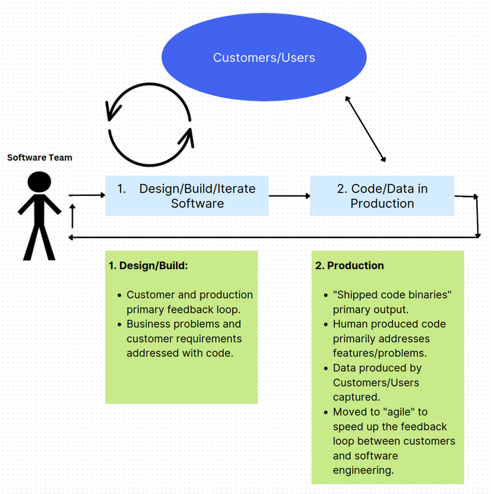
- Software team analyzes customer requirements and problems. Types code into an editor, compiles it, tests it, and ships it to production.
- Customers/Users use software in production, generating data for their domain, and telemetry for the software team to analyze.
There are two feedback loops here: one between the software team and the customer, and another between the software team and telemetry gathered from production. Improvement in the product or system requires a human in the loop to engineer extra things, and subsequently requires a deployment to production.
Some observations of these feedback loops:
- This software development life-cycle has been fairly linear for decades, with some velocity improvements coming from programming language, tooling, and process improvements.
- Silicon Valley’s “Move fast and break things”, increased this feedback loop up by moving to continuous deployment and production based A/B testing.
- That (b) was enabled through the age of ultra connectivity (mobile etc) and wide and immediate distribution.
Adding ML to the software engineering domain affects this loop:

- ML Engineers/Researchers identify features/problems in the product which a) can be learned by a machine to solve in a higher value way than humans or code, and b) can be improved over time automatically by capturing user or machine generated data and injecting that into the model’s “training loop”.
- The trained model is deployed into production and can be called like a library or API from the software/product. These models are either refreshed often, or continuously trained near real-time.
There is an important difference between software engineering without ML (first figure), and software engineering with ML: the first depends on a human in the feedback loop to produce more value for customers over time, and the second has a machine in the feedback loop. A machine in the feedback loop enables a) product and engineering scale beyond the total capacity of the team of humans, and b) will usually end up being non-linear.
It’s worth spending a few moments on why non-linear value generation will be powerfully disruptive, and why machine learning tends to have an exponential looking value creation curve.
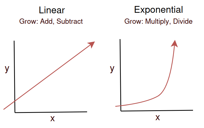
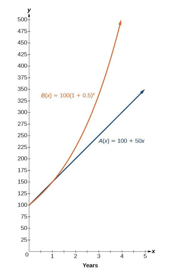
A quick reminder that Linear models represent a fixed increase in ‘y’ for every ‘x’, or said another way, we “add” an increase of growth ‘x’. In an exponential relationship between ‘x’ and ‘y’, for every step of ‘x’, the growth rate accelerates rather than staying fixed:
(Would you rather have a business that ‘adds’ a fixed step of growth output per year, or has an increasing step of growth output per year?)
Imagine you have a simple spam filter that works on a set of rules written by developers. For instance, if an email contains the word “lottery” or “prize”, it marks it as spam. So, each time you want to add a new rule, a developer has to write it. If you have 10 rules, you might catch X% of the spam. Add 10 more rules, and you might catch another X%. This is a linear relationship between effort and outcome. The function might look something like:
Spam caught (%) = 0.005 * number of rules + initial_model_baselineOn the other hand, let’s say you train a machine learning model on a dataset of spam and non-spam emails. Initially, with a small amount of data, the model might not perform well. But as you add more data, the model’s performance. This relationship can be modeled with a logarithmic function, which is a typical example of a non-linear function:
Spam Caught (%) = 100 * log(Data Size)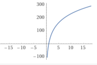
So with a small data size, the model doesn’t catch much spam, but as the data size increases, the performance improves significantly (though it begins to plateau eventually).
In this case, data availability drives non-linearity. However there are several other contexts under which machine learning will tend to generate non-linear effects:
- Model complexity: more complex models may improve performance of tasks, or enable step changes in coping with task complexity.
- Computational power: similar to data availability, the benefits of additional computational power and longer training times can have a non-linear impact on task outcome.
- Model cooperation/chaining (model stacking, ensemble learning etc): combining or chaining models together to complete tasks more precisely or to allow for increased task complexity.
- Model introspection and self-instruction: (see later in the Large Language Model section).
Capturing this value generation requires more sophisticated engineering teams right now, but I imagine as tools improve and abstractions are built, this cost and complexity will come down.
Using/Extending/Fine Tuning Existing Models
Once models are trained, they can be shared with others, allowing users to avoid the upfront cost of training. This can be done by either sharing the model binary (typically megabytes to hundreds of gigabytes), or by calling a cloud hosted model through an API. Cloud hosted models are popular distribution mechanism for large language models in particular, given their size (hundreds of gigabytes), their cost (, and how often they’re being updated.
Model binaries can be extended and fine-tuned, allowing consumers to build on or tweak model capability. “Extension” of a models capability can be done in many ways, but a popular way is to combine the model with other models – either by chaining together the inputs and outputs of each model to solve a task, or by blending the outputs of many models together (allowing the models to essentially ‘vote’ on the task outcome).
“Fine-tuning” a model can also be done several ways, but a popular choice among large language model fine-tuners is to take an existing open weights LLM like Llama, add a few extra layers before the “output” layer, and continue training the overall model. Training will end up focusing those last few layers on building specialization to solve for the tasks provided in the fine tuning. Fine-tuning requires just fractions of the training capacity and training time.
The best place to find existing ML models (either source code, binary files or both) or fine-tuned models is HuggingFace, (essentially “GitHub for ML”) which hosts thousands of models and datasets for download.
LLMs “in the loop”
The above few sections talks about ML “being in the loop”, with particular reference to the software engineering development lifecycle, and how that kicks off higher velocity, non-linear value creation. But there’s an even stronger version of this - a view widely held by frontier LLM labs - that as LLMs progress towards AGI, all software engineering tasks that are required to create and kick off that loop will be performed and automated by LLMs themselves: they’ll both build the loop and be inside the loop.
One implication for this stronger version is that the software development lifecycle itself becomes exponentially more efficient. Instead of humans writing code to create ML feedback loops, LLMs will:
- Analyze business requirements and automatically design appropriate ML architectures, or simply use themselves as the model of choice.
- Generate the code for data pipelines, model training, and production deployment
- Monitor model performance and autonomously improve both the models and the surrounding infrastructure
- Create and manage the feedback loops that enable continuous improvement
The practical consequences of this are profound:
- Development velocity will increase by orders of magnitude as LLMs can work 24/7 and parallelize across multiple tasks
- The quality of ML systems will improve as LLMs can analyze patterns across thousands of deployments and apply best practices
- The cost of building ML-powered systems will dramatically decrease, democratizing access to sophisticated AI capabilities
- Businesses can focus on defining problems and desired outcomes, while LLMs handle the entire implementation stack
This represents a fundamental shift from current practices where humans are the bottleneck in the software development process. The transition will likely follow a pattern where LLMs first assist human developers (current state), then handle routine development tasks (near future), and finally manage entire ML pipelines autonomously (future state).
For businesses, this means that competitive advantage will increasingly come from:
- The quality and uniqueness of data they can provide to LLMs
- Their ability to clearly articulate business problems and success criteria
- How effectively they can integrate LLM-driven development into their operations
Building Machine Learning Engineering Teams
| Title | Level at FAANG | Compensation /Year |
|---|---|---|
| Machine Learning Researcher (Senior) | E8-E9 | $2-4 million USD |
| Machine Learning Researcher (Mid) | E6-E7 | ~$1-2 million USD |
| ML Engineer (Applied ML) (Senior) | E8-E9 | ~$2-3 million USD |
| ML Engineer (Applied ML) (Junior-Mid) | E5-E7 | ~$500k-1.5 million USD |
| Software Engineer (with ML Experience) | E6 | ~$600k-1 million USD |
| Software Engineer ML Infrastructure | E6 | ~$600k-1 million USD |
Outside of the US, the market is a fraction of the cost. As a guess, Australia, the UK and Europe are likely 2-5x cheaper for similar talent.
Hiring is competitive and expensive. Re-skilling in-house talent may be a better strategy long term, particularly as abstractions and automation of ML model development will likely be bridged with skills that software engineers already know. This bridging will happen over the next 12-36 months. Given AI product integration is inevitable, and AI talent will be required for that, the highest impact question to answer is timing - when and how do we evolve our teams?
Some questions to help ponder timing:
- Can any of the models listed in “Examples of AI in action” be strung together by competitors to build product differentiation or competitive advantage?
- Are there existing customer problems where models listed in “Examples of AI in action” can help solve?
- How fast can the engineering/business culture adapt to team composition shifts.
You can get your current teams preparing for ML now:
- Do we have the data? Given AI/ML models thrive on data, data is a significant input into building a machine learning value flywheel. If we don’t have the data, can we instrument our products or process to get it?
- Data lineage will be important: when regulation inevitably lands, regulators will want to know where the data used to train the models came from. Tooling and instrumentation here is critical.
- Capacity planning: multiple factors more hardware capacity will be required to do ML ops properly (regularly retraining models, generative training data, etc).
- Identifying how user experience expectations will change in the face of AI everywhere.
- Have your current engineering team do “deep work” and experimentation with frontier LLMs.
Bibliography
TODO
Author
I previously worked at a FAANG on scaling AI infrastructure and the AI software stack. I now work at a frontier LLM company. You can contact me here: https://9600.dev