Thoughts about AI for Investors, Decision Makers and Managers
This document aims to provide: 1) a high-level understanding of Artificial Intelligence/Machine Learning, 2) predictions on how it will impact software engineering and product development, and 3) explain my mental model for AI investments.
The key takeaway: AI generates non-linear effects on deployed systems/ecosystems, enabling non-linear capital returns. Investors should:
- Identify and exploit opportunities where ML generates non-linear effects (and returns).
- Understand how ML works and the feedback loops required for non-linear effects.
Understanding (2) is crucial for skillfully spotting opportunities in (1).
Vocabulary: AI, Artificial Intelligence, and Machine Learning are used interchangeably. ‘AI’ broadly encapsulates technology and products, while ‘Machine Learning’ refers to machines learning from data.
Examples of AI in Action⌗
Let’s tour the AI technology and product landscape before trying to build a high level understanding of how it works. You can skip this section if you’re familiar with products and model types.
Models, Model Type: described in the “What is a ML Model” section. A model is the output of a machine learning process.
| Model Type | Tasks |
|---|---|
| Object detection, tracking | Identifying/tracking objects, scenes or people in images and video. Making predictions on objects locations/trajectories. Demo |
| Speech | Cloning, tuning, speech to text, etc. Demo |
| Text Translation, Classification | Language translation, sentiment analysis etc. Demo, Demo |
| Recommendations | Search engines, YouTube recommendations, etc. Demo |
| Games, Game Theory | Game engines, combatants, etc. Demo, AlphaStar Starcraft II |
| Generative | Text generation, chatbots, ChatGPT, music generation etc. Demo |
| Optimization | Compression techniques, generated code optimization, game engine up-scaling, etc. |
| Creative | Sketches to imagery, auto video generation, diffusion. Demo, Demo |
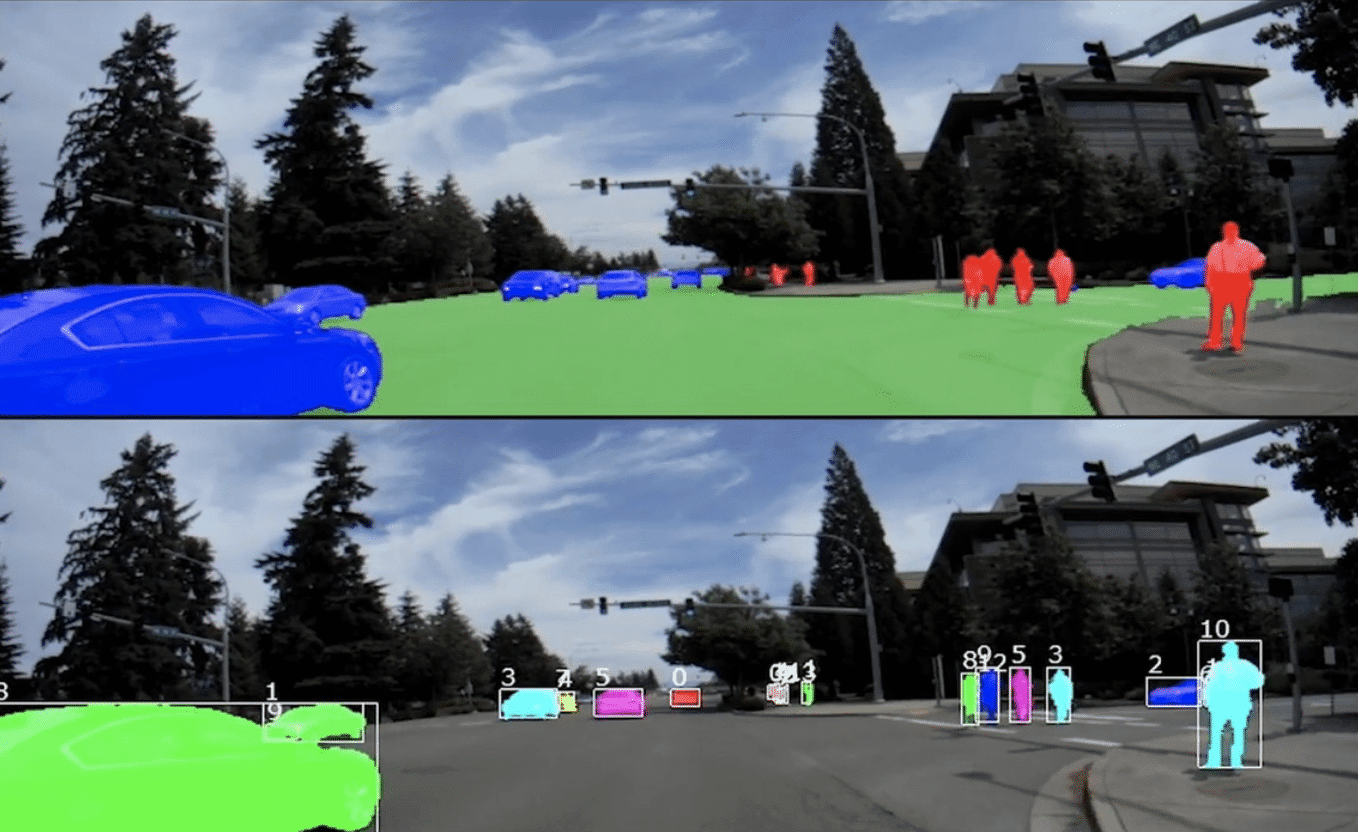
Object detection, tracking and segmentation⌗
State of the art (SOTA) now includes high fidelity segmentation (bounding boxes) and the ability to track those segmentss across frames.

Speech⌗
SOTA features include: speech-to-text recognition of hundreds of languages (used for YouTube closed captions); flawless text-to-speech (useful for Audiobooks etc); speech enhancement; lip reading;

Text Translation and Classification⌗
SOTA features/tasks include: Summarization, retrieval, classification, question answering, common sense reasoning, abuse detection, sentiment analysis, emotion analysis.

Generative⌗
Features/tasks include: text-to-image generation, general AI chat-bot interactivity, text-to-video generation etc.
-
- text-to-image generation
a portrait of an old coal miner in 19th century, beautiful painting with highly detailed face
-
- Midjourney images

- Midjourney images
-
NVIDIA - High-resolution video synthesis with latent diffusion models
-
a teddy bear painting a portrait
-
Gen-2 Runway (StableDiffusion text to video):
- “Beautiful creatures swimming under sea”

- “Beautiful creatures swimming under sea”

Applications⌗
SOTA: Game playing, protein folding,
-
AlphaStar: Mastering the real-time strategy game Starcraft II

-
AlphaFold: predicting 3D models of protein structures for biological research acceleration

-
Findsight.ai - find thousands of core ideas from non-fiction works

The list for what machine learning models are capable is a) far too long, and b) getting longer every week. The best places to see where machine learning model innovation is happening are:
- Hugging Face - Open Source/Downloadable Models
- Two minute papers YouTube Channel - understand new ML model research quickly.
- Reddit /r/MachineLearningNews
The basics of how ML works⌗
Now that we’ve had a look at the top-down capability of machine learning/AI from a model and product perspective, we will start the journey to understand the basics of how machine learning works under the hood.
What is an ML Model?⌗
There are well articulated definitions of what machine learning models are on the Internet, so I’ll say that models are essentially a piece of software that takes data as an input, and makes a prediction as an output in a domain we care about. Models are trained by looking at lots of input examples, trying to guess the output, and when there is error, the model updates itself to be less erroneous next time. Given enough examples, the model will be more precise, and hopefully general enough to give accurate predictions on input it has not seen in training.
This concept is unlikely a surprise, as we’ve been using “machine learned” models in tools like Excel for years. And ironically, one of the easiest Excel modeling techniques, Linear Regression, is the fundamental building block for how machine learning works in the large.
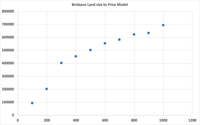
A quick recap of Linear Regression: We’ll build a simple Linear Regression model to predict house prices. Let’s take some historical price data, which I’ve plotted below (x axis is land size in square meters, and y-axis is the price):
Asking Excel to generate a Linear Regression model with a couple of clicks gives me a nice red line, and a function representing the linear model:
y = 603x + 139333
Where y is the house price prediction, and x is the land size input.
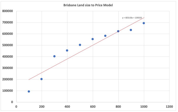
How Excel calculates this line is an exercise for the reader (start here), but we will steal the equation and the red line to explain how the learning part happens in machine learning.
To figure out the best fit line, we start with a random number to multiply land size in our linear model:
y = random() * x + c, or:
price = random() * land-size + y-intercept
So for random(), let’s assume it generated 300 as its random number (and we’re going to ignore the y-intercept for now):
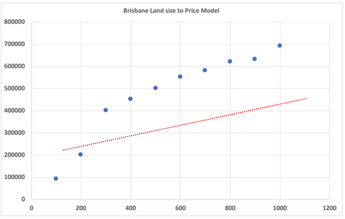 Not terribly close to reality, so let’s bump the random() number up, so that line gets a little steeper:
 y = 350 * land-size
 Better!
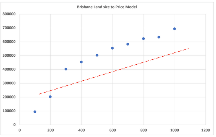
Now we’re going to repeat the “tuning” of that variable until the line has the least amount of “error”:
350 -> 450 -> 550 -> 650 -> 610 -> 603!.
price = 603 * land-size
And that’s it. We’ve learned the most appropriate variable with the least amount of error is “603”, such that price = 603 * land-size.
Before we move on, let’s go through the vocabulary definitions as they relate to machine learning for the example we’ve just seen:
- The initial number we used for random() to adjust the slope of the line, in ML terms that’s called a “parameter” or “weight”. (In Linear Regression terms, it’s call the coefficient). This is the “heart” of the model, as it has the biggest influence on the slope of the line.
- The “x” axis variable (Land Size) is called an “input parameter”. It’s the thing we give the model to make a prediction on.
- The loop of:
- Make a model with a “parameter” or “weight”
- Check the model against existing data
- Calculate the error
- Bump the “parameter” closer to ensure a less erroneous fit for the data we’ve seen
- This is called the “training loop”.
One parameter models can only generate straight lines, which isn’t terribly useful particularly when we have data that is non-linear:
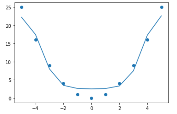
From one parameter to many⌗
Scaling this to multiple input parameters is as simple as extending the model to represent non-linearity, which mathematically looks like:
$$ \begin{aligned} y = P_1x_1 + P_2x_2 + … + P_nx_n \\\ \end{aligned} $$
There are multiple P or parameters, multiple x, which are the inputs (or input parameters), and y which is the predicted result, or thing we’re trying to learn. The training loop above still applies, we’re going to be nudging a lot more parameters in order to reduce the error now.
In the example above where the data looks like a parabola, we’ll need several model parameters in order to fit that data properly. The wonkier the data, the more parameters we need. In fact, Large Language Models have 10’s of billions of parameters in order to learn the underlying patterns in the data it is fed.
Deep Learning⌗
You may have seen some diagrams of Neural Networks, or Deep Neural Networks. These diagrams are a graphical representation of a much larger calculation that uses the equation above as its fundamental building block.
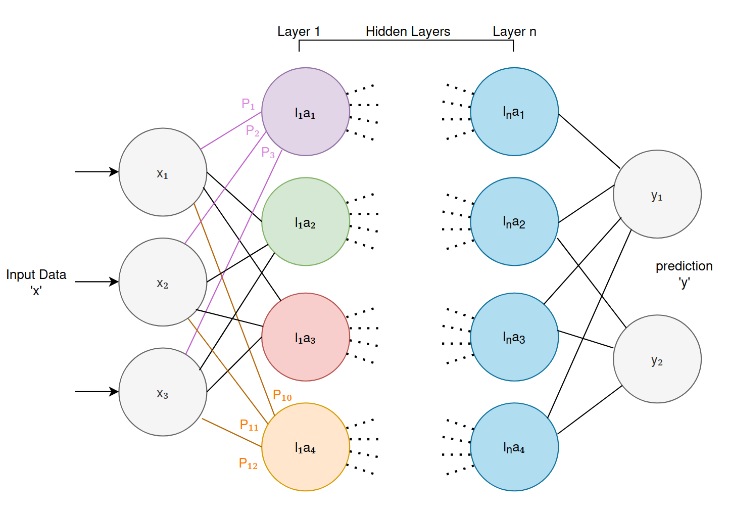
At a really high level:
- Each of those colored circles are “neurons”.
- Each neuron receives “data” from any connections to other neurons it has to its left. The biological equivalent being “synapses”.
- Each of those data are multiplied by ‘parameters’ or ‘weights’ and then summed up. Essentially calculating the equation we saw above:
$$ \begin{aligned} l_1a_1 = P_1x_1 + P_2x_2 + P_3x_3 + P_4x_4 \\\ \end{aligned} $$
- Which generalizes to:
$$ \begin{aligned} l_na_z = P_1l_1a_1 + … + P_zl_na_z \\\ \end{aligned} $$
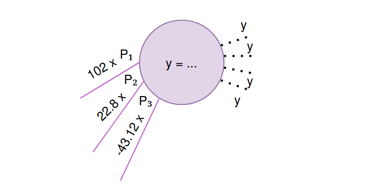
- Don’t let the math symbols worry you. Just think of every neuron computing the ‘y =’ linear equation from above. We take variables in, multiply them by parameters and produce a result for the next neuron. It might look like this:
- If the end result of this chain of ‘y =’ computation doesn’t produce the right result (error), we ’nudge’ all of the parameters for each neuron to get those neurons to be better at collectively producing the right result.
- The more neurons, parameters, and layers there are, the more “non-linearity” and space for the model to learn and fit the data properly.
And with that, we’ve just learned that you can go from a single line linear regression ‘fit’, to a non-linear fit by just composing together the same basic linear equation over and over again.
There’s three more concepts to learn and then we’ll have a solid high level understanding to use to explore the strategy of the machine learning space: 1) how input data is represented, 2) what are layers, and what are they learning, and 3) how these neural networks are represented and calculated using matrix math.
Input and Output Data Representation⌗
The “input data”, “input layer”, or the “x1 .. xn” is always encoded as a number, so a question that regularly comes up is “how are images, video, documents etc, represented in the input”. They’re converted to their numeric representation:
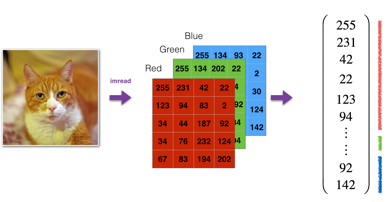
Here, every pixel is converted to it’s red, green, blue value and those values are used in the input layer. This implies that big images with tens of thousands of pixels, will be fed to a neural network model that has tens of thousands of input neurons, and will require tens of millions of parameters to allow the model to learn!
The concept is the same for video, text, and so on. Everything is converted to a number and fed in to that first “input layer”. Text for example, can be encoded using a simple character to number encoding:
a = 1b = 2c = 3- …
Hidden Layers⌗
The ‘hidden layers’ that are shown in the deep learning diagram above have a magical property: through the mathematics of “nudging” parameters in the training loop, hidden layers and their neurons end up ‘specializing’ on smaller tasks within the overall task of predicting an output.
Let’s unpack that dense sentence with a diagram:
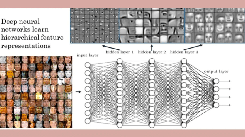
Here we’re trying to learn something about human faces (perhaps we’re trying to predict the mood of a face out of four different moods: happy, sad, neutral, angry). We feed the machine learning model lots of pictures of faces, and ask it to predict mood.
In order to perform that task, the model needs to learn skills that will help it better predict mood: what are the mouth and eyes doing, squinting? angled? etc. And in order to perform that overall task, the model will need smaller specialty skills, like finding edges in an image, finding contrast, identifying mouth, nose, eyes, and so on. If you look closely at the image above, you can see each hidden layer learning to perform those specialist tasks.
You can think of the “output layer” as asking the previous layer (the last hidden layer) for its judgment on the task that it’s a specialist in. That layer then asks the previous layer for its judgment, and then that layer asks the previous layer, and so on and so on.
This kind of implies that more layers means more specialties, allowing the model to perform more and more complex tasks. Too few layers, means the layers can’t break down problems into smaller tasks, and that may mean that output predictions are poor: just not enough collective expertise in the model.
This kind of intuition on how models are learning extends to even the most complex models, like Large Language Models. You can imagine the last layer “I need to produce some text to respond to the input text I’ve been given” as that layer essentially asking all the previous layers (the experts) to work together to craft an appropriate answer.
Matrix Multiplication⌗
The magic above of taking data and pushing it through many layers requires a massive amount of mathematical calculation. Computers are generally pretty good at calculating this kind of thing, but one piece of hardware in a computer is exceptionally good at it: graphics cards. The kind you would buy to run the latest and greatest games at the highest graphics settings. Getting from what a deep learning model looks like to running on a graphics card (GPU) is done through high school linear algebra and matrix math.
The following shows the neural network example above, and shows how those calculations can be performed using matrix math:
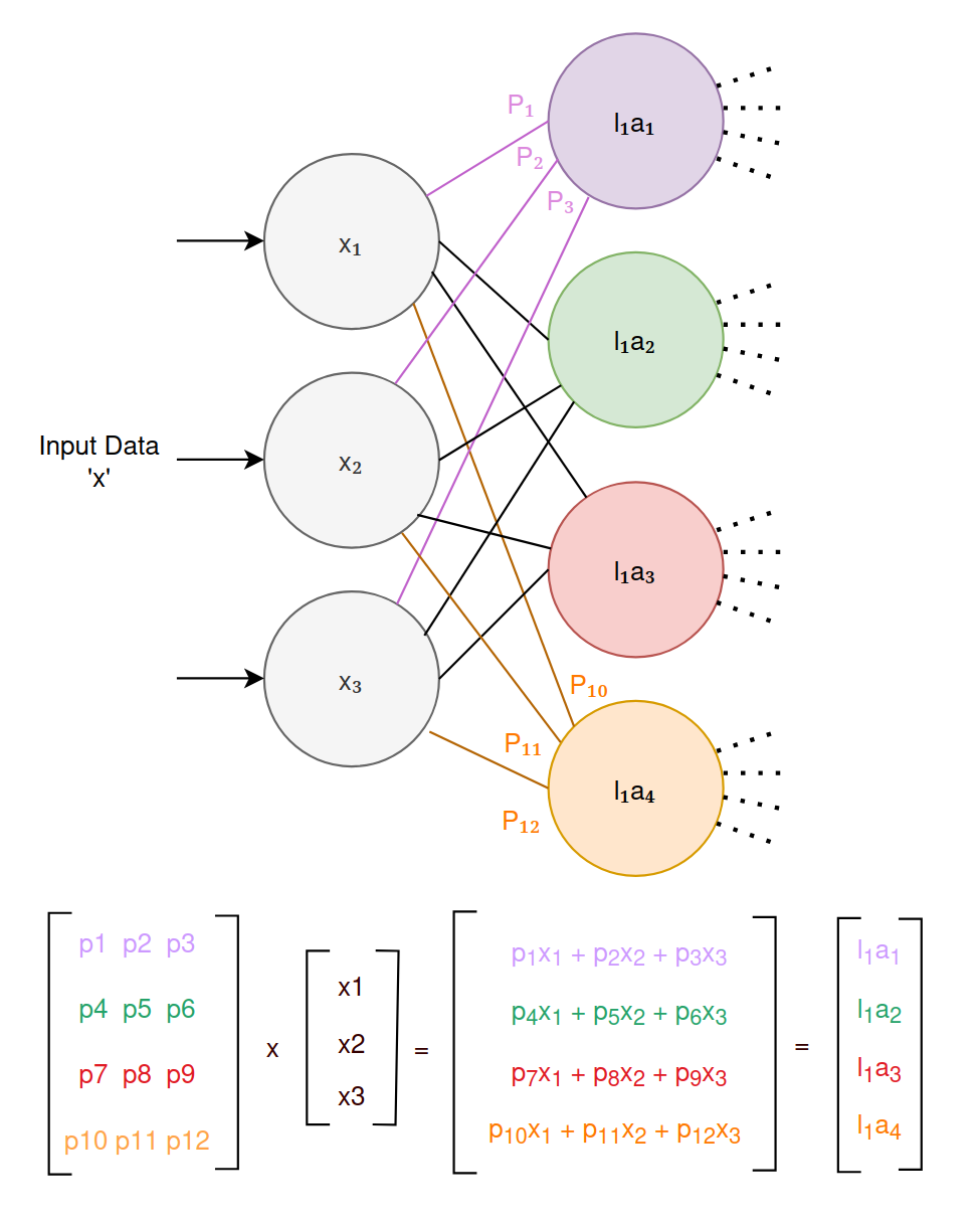
It’s not important to understand how this calculation works in detail, just that it can be represented and calculated using matrix multiplication.
This idea of using matrices to represent and calculate is important, as it explains why Graphics Processing Units are so excellent at building and training these big models: GPUs have been crunching matrix math for years. All those 3D games you play represent their visual scenes as polygons, the underlying representation being matrices! Rotating, flipping, clipping matrices is well known matrix math that has been optimized really well in the GPU hardware already – it’s perfect for deep learning.
What GPU hardware looks like and what it costs is detailed further down in the paper. For now, just think “deep learning equals matrix math which runs great on GPUs”.
Models as Code⌗
Let’s take a quick look at what machine learning models look like as software code. There is one dominant library/framework for using, building and researching machine learning models: PyTorch, which runs on the Python programming language. The distant second is Google’s TensorFlow. There is a long-tail of other libraries and frameworks for various programming languagues, but its the authors belief that deviating from the PyTorch ecosystem makes little sense as of 2023:

The code below will show a PyTorch neural network model that will train and learn how the XOR (eXclusive OR) truth table. The details of how the code is run isn’t important, as we’re just trying to visualize the structure/example of a neural network model:
| A | B | A XOR B |
|---|---|---|
| 0 | 0 | 0 |
| 0 | 1 | 1 |
| 1 | 0 | 1 |
| 1 | 1 | 0 |
import torch
import torch.nn as nn

class XOR(nn.Module):
    def __init__(self):
        super(XOR, self).__init__()
        self.input_layer = nn.Linear(2, 2)
        self.sigmoid = nn.Sigmoid()
        self.output_layer = nn.Linear(2, 1)

    def forward(self, input):
        x = self.input_layer(input)
        x = self.sigmoid(x)
        y = self.output_layer(x)
        return y
The code above is a PyTorch neural network model definition, with two input parameters, and one output.
xs = torch.Tensor(
    [[0., 0.],
     [0., 1.],
     [1., 0.],
     [1., 1.]]
)

y = torch.Tensor([0., 1., 1., 0.]).reshape(xs.shape[0], 1)
This code represents the training data that PyTorch will use to train the model above.
if __name__ == '__main__':

    epochs = 1000
    mseloss = nn.MSELoss()
    optimizer = torch.optim.Adam(xor.parameters(), lr=0.03)
    all_losses = []
    current_loss = 0
    plot_every = 50

    for epoch in range(epochs):
        # input training example and return the prediction
        yhat = xor.forward(xs)

        # calculate MSE loss
        loss = mseloss(yhat, y)

        # backpropogate through the loss gradiants
        loss.backward()

        # update model weights
        optimizer.step()

        # remove current gradients for next iteration
        optimizer.zero_grad()

        # append to loss
        current_loss += loss
        if epoch % plot_every == 0:
            all_losses.append(current_loss / plot_every)
            current_loss = 0

        # print progress
        if epoch % 500 == 0:
            print(f'Epoch: {epoch} completed')
The code above is the training loop.
# test input
input = torch.tensor([1., 1.])
print('XOR of [1, 1] is: {}'.format(xor(input).round()))
This code tests the model once it’s been trained. Running this code produces the following:
The result is XOR of [1, 1] is: 0
A more complex example that is both interesting, and reasonably trivial to train is having a neural network learn how to play the Nokia phone game “Snake”. This example uses a model architecture and training procedure called “reinforcement learning” – the training loop essentially plays millions of games of Snake, trying to learn the best strategies.

Code can be found here. GIF demo (after 10 minutes of training):

Size of Models and Time to Train⌗
Training the XOR model is a trivial task, taking milliseconds. Training larger more complex model architectures can take months. Training time and training complexity is typically dependent on 1) how many parameters in the model need to be ’nudged’, 2) how much training data is required to have the model learn in a generalized repeatable way, 3) the model architecture used. There are more, but this is a high level rule of thumb. Some examples of training time, model size and compute required:
| Model | Training Time | Size | Compute |
|---|---|---|---|
| XOR | Milliseconds | 4 parameters | Laptop |
| Snake | Minutes | 12 parameters | Laptop |
| MNIST Digit Classification | Hours | 100-300 thousand | Laptop |
| ImageNet image classifier | 15-20 hours | 25-150 million | Desktop |
| YouTube Ranking and Recommendation | Weeks | Billions | Server Farm |
| ChatGPT Language Model | Months | 100s billions |
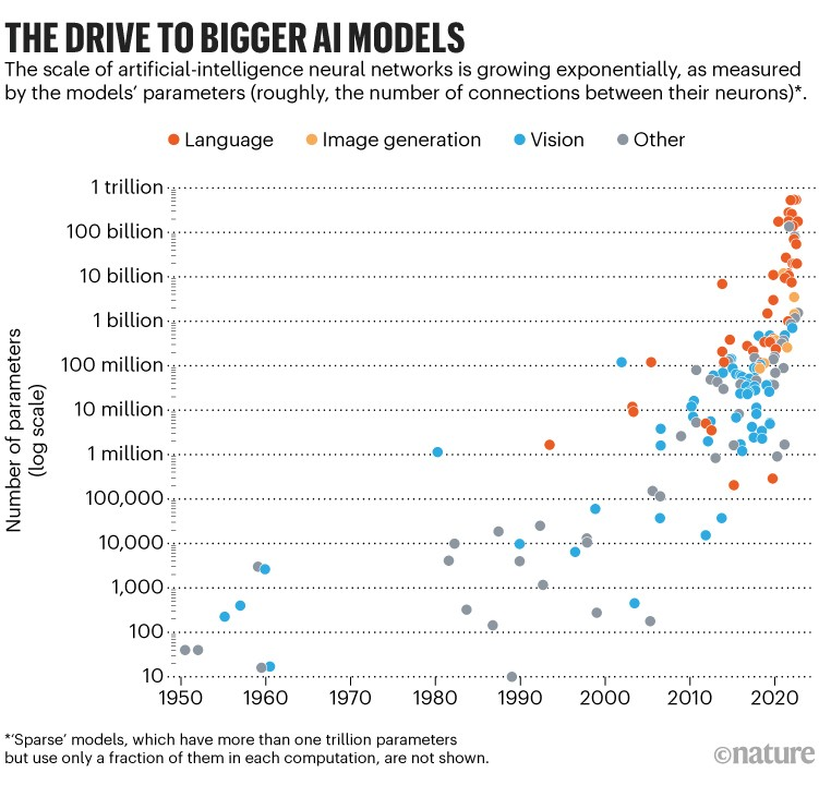
Nature has good graph that represents the exponential scale of new machine learning models and research:
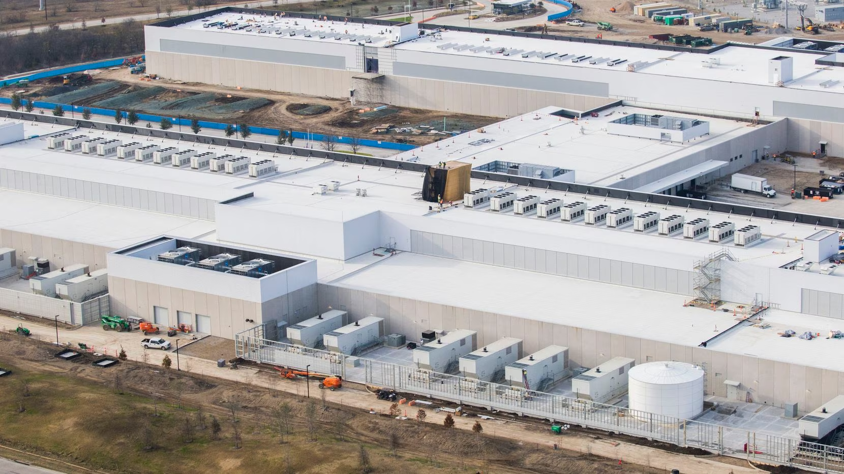
The compute required to train the largest and most complex models (right now, language models like ChatGPT) is large and expensive. The following pictures give a sense of scale:
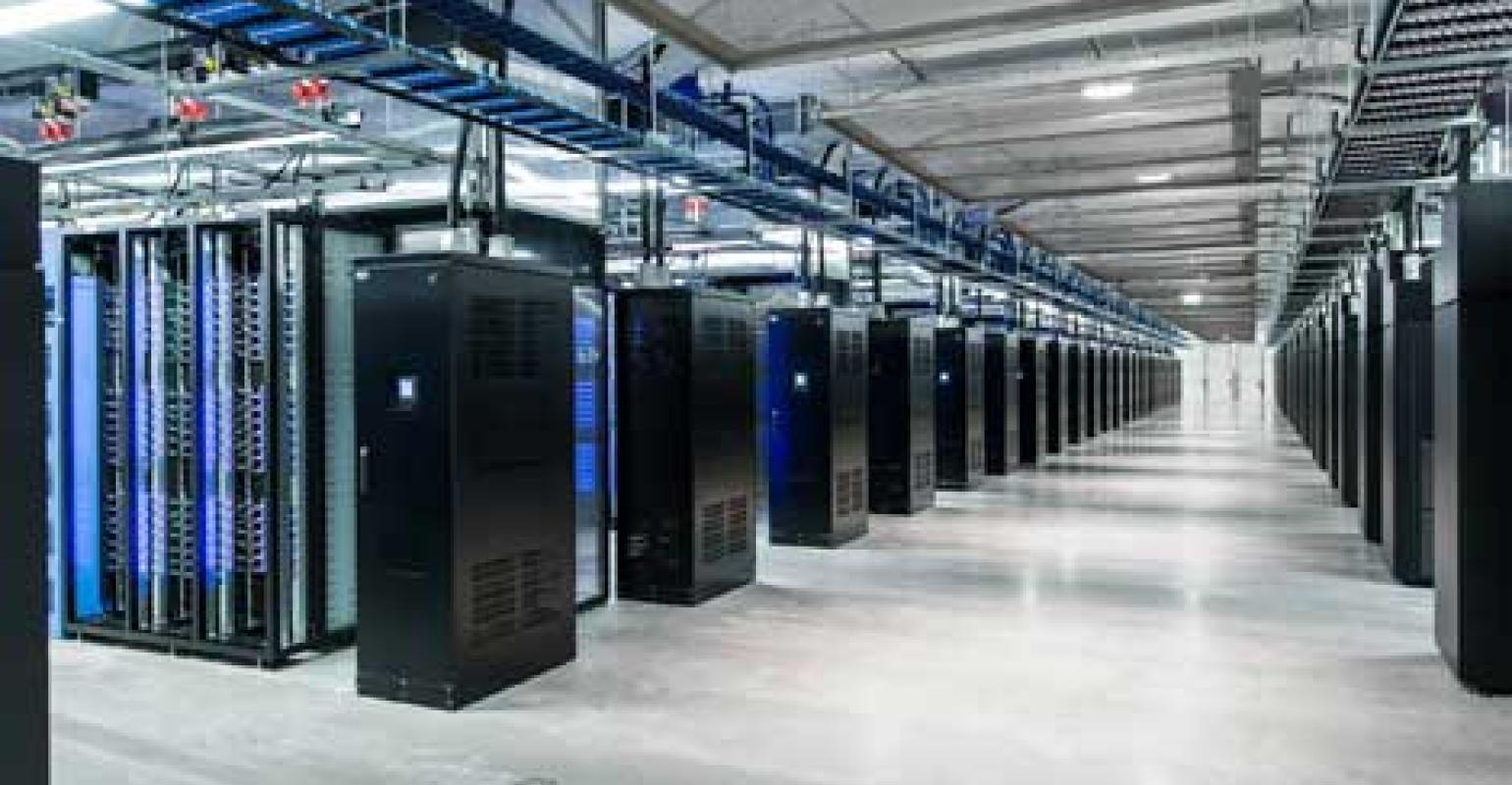
-
Facebook’s Fort Worth Data Center (2 full data center buildings):
-
Inside the data center:
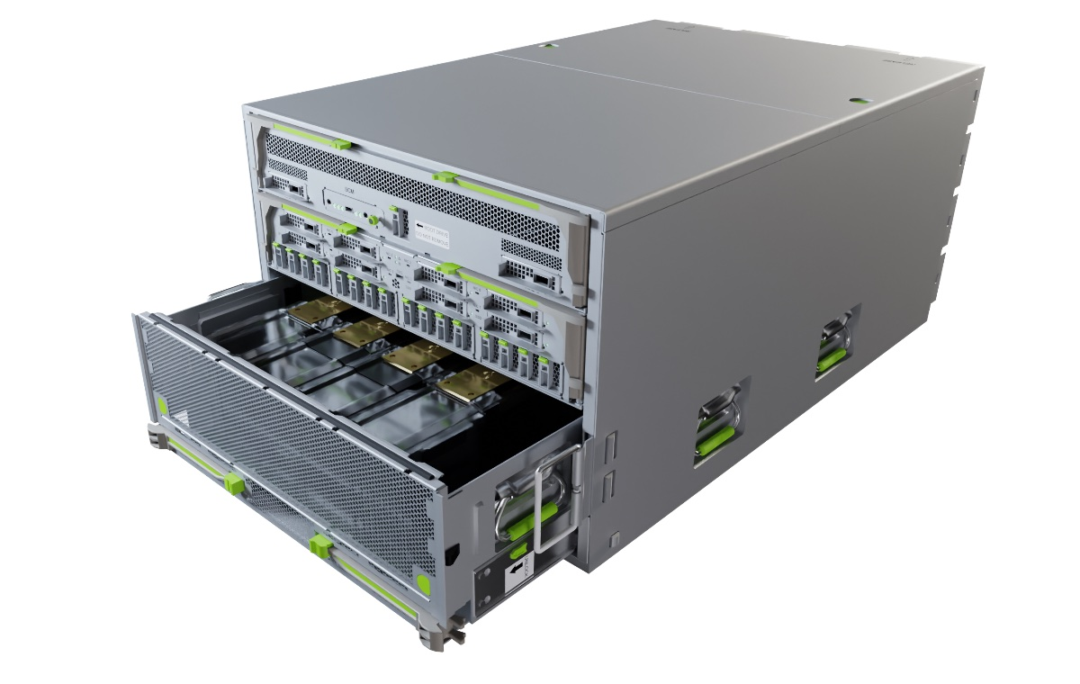
-
Rack based NVIDIA GPU Server, “Grand Teton” from Meta. Approximately 8x NVIDIA H100 GPU cards, ~15kw per rack typically:
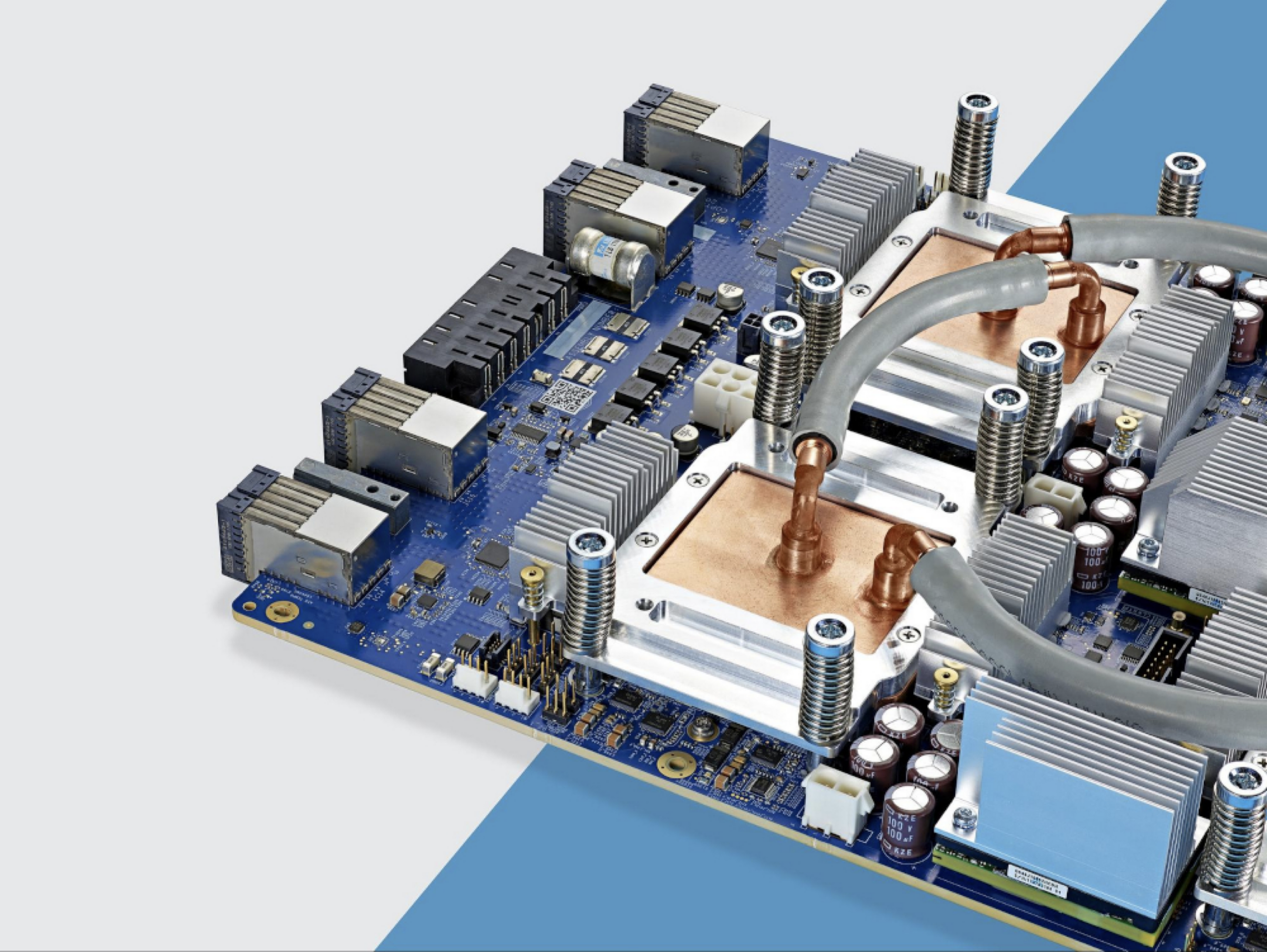
-
Single H100 NVIDIA GPU (Latest Generation 2023). ~800W power draw. Selling for ~$27k on eBay right now.

Exactly how many GPUs are required to train these latest super models like ChatGPT is an industry secret, but it’s understood that tens of thousands of GPUs were required for training, and more for serving the finished model to the millions of customers that use it.
Google, Meta, Amazon and Microsoft have hundreds of thousands of GPUs available to machine learning researchers/practitioners to experiment on, build, and train models for production use.
In general, more compute is a competitive advantage:
- Researchers can explore bigger and more complex model architectures to achieve learning of more complex tasks.
- Higher velocity of output of research and model experimentation: faster equals more experiments
- Global scale deployment of complex machine learning models for your customers/users.
Machine Learning “Accelerator” Hardware⌗
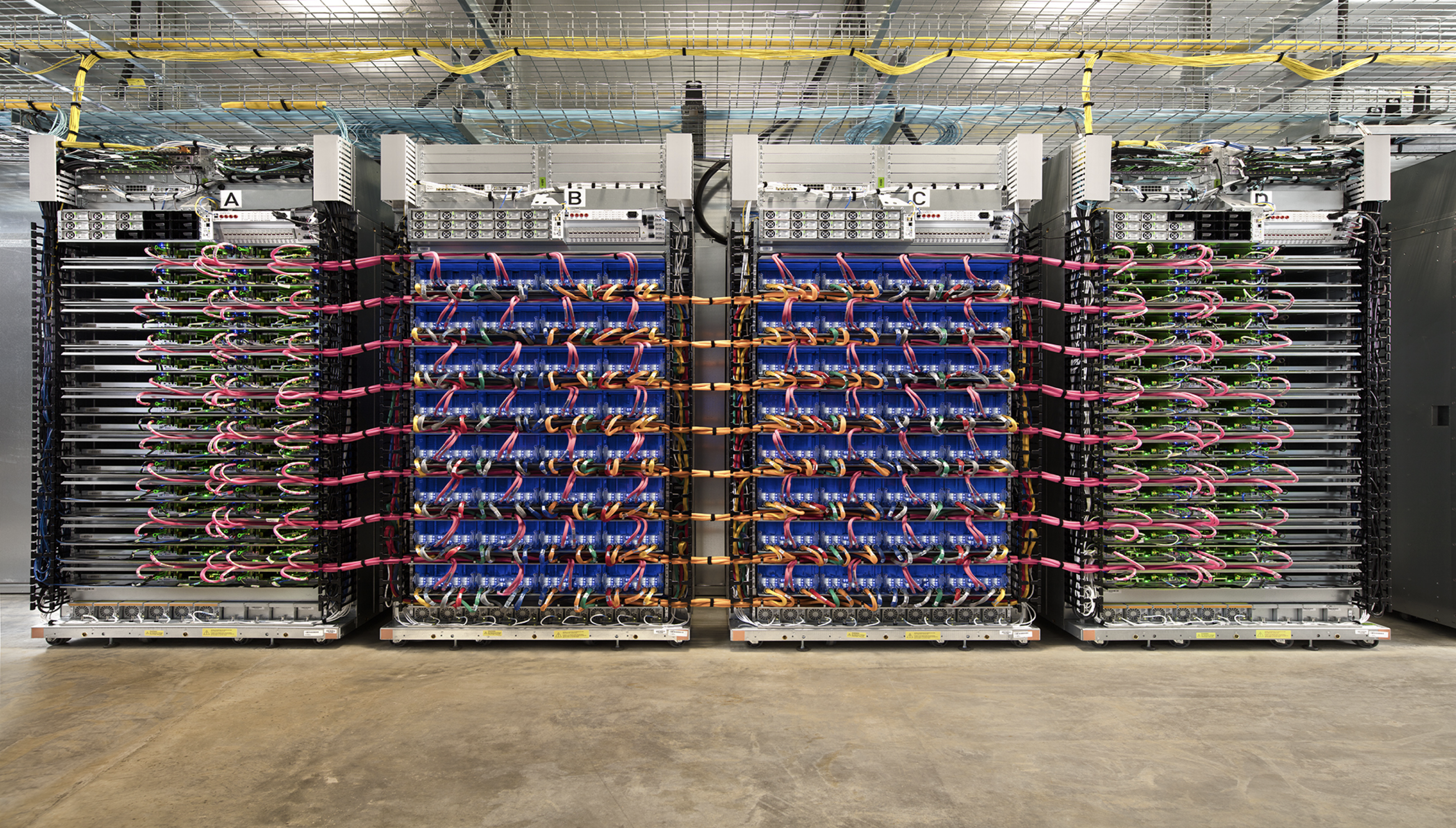
You may have heard about specialized hardware that hyperscalers like Google have built, an example being Google’s “TPU”. This hardware looks and acts very similarly to GPUs, but may have a different configuration (compute, available RAM, connectivity to other TPUs etc) that may be more specialized to a particular type of model.
Here’s a picture of a TPU (the plastic piping is used for water cooling), and another picture of many TPUs connected together in a data center rack:
There’s a view here that specializing hardware to models may mean bigger, better, and faster trained/productionized models. I’m skeptical of this claim for numerous reasons that are beyond the scope of this paper. This hardware exists, companies pitch it as a competitive advantage, and you should know about them, but that’s about it at the limit.
Costs⌗
Optimization and cost savings for training and deploying machine learning models has become critical. In general, FAANG’s, large enterprise, and cloud providers are optimizing for the following things:
- Performance per/ $Dollar (floating point operations per second, or how many matrix multiplications can be performed) for given capital expenditure cost of hardware.
- Performance per/ Watt (energy usage per floating point operations). Power can be a dominant planning constraint for data center build outs.
- Machine Learning Researcher/Engineers experiment, build, measure, test, deploy loop.
- Data preparation and labeling.
Optimizing (1) and (2) can be achieved in numerous ways:
a. hardware vendor choice b. hardware vendor software stack c. limiting/refining/curating training data (thus reducing how long training takes) d. trading off model accuracy by reducing training time e. model architecture choices (decreasing parameter count, alternative choices in model architecture, etc) f. software optimizations (purchasing libraries that improve the performance of training and serving) g. compressing models (a technique called quantization, which trades off accuracy for parameter size) h. reducing “freshness” of the model (reducing how often you re-train the model) i. using “off the shelf” models instead of training your own.
Creating a strategy for constraining costs is more art than science right now, as ‘a’ through ‘i’ are often difficult to measure, and difficult to connect to product/customer impact.
Costs to train and deploy will differ depending on:
- the complexity of the model being trained/deployed
- how many end-users are using the model in production
- how often the model needs re-training
- from scratch training, or fine-tuning/extension from existing model (see below).
The “Size of models and time to train” section above gives a general sense of training compute requirements. Deployment (or “inference”) requirements can vary and depends almost entirely on the size of the customer base that will use the model at any given point in time.
Optimizing (3) and (4) is talked about later in the paper under Developer Experience and Operations.
Using/Extending/Fine Tuning Existing Models⌗
Once models are trained, they can be shared with others, allowing users to avoid the upfront cost of training. This can be done by either sharing the model binary (typically megabytes to hundreds of gigabytes), or by calling a cloud hosted model through an API. Cloud hosted models are popular distribution mechanism for large language models in particular, given their size (hundreds of gigabytes), their cost (, and how often they’re being updated.
Model binaries can be extended and fine-tuned, allowing consumers to build on or tweak model capability. “Extension” of a models capability can be done in many ways, but a popular way is to combine the model with other models – either by chaining together the inputs and outputs of each model to solve a task, or by blending the outputs of many models together (allowing the models to essentially ‘vote’ on the task outcome).
“Fine-tuning” a model can also be done several ways, but a popular choice among large language model fine-tuners is to take an existing LLM, add a few extra layers before the “output” layer, and continue training the overall model. Training will end up focusing those last few layers on building specialization to solve for the tasks provided in the fine tuning. Fine-tuning requires just fractions of the training capacity and training time.
The best place to find existing machine learning models (either source code, binary files or both) is HuggingFace, (essentially “GitHub for ML”) which hosts thousands of models and datasets for download.
Core Concepts⌗
From here, we’ll raise the level of abstraction up a few levels for the rest of this paper and talk mostly about four building blocks, “Data”, “Model Architecture”, “Task”, and the “training loop”:
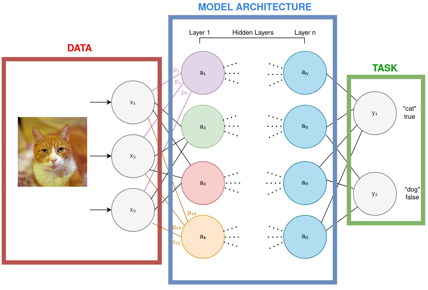
- Data: the inputs used to train the model to perform the task. These can be any sort of media these days: images, video, sensors, environment, database data, etc.
- Model Architecture: the size and shape of the model. We’ve looked briefly at Deep Neural Networks and it’s underlying equation and how it learns, but there are various shapes and sizes of both the equations one uses, and how the learning gets performed. Architectures vastly impact the performance of the task, and how cheap/expensive it is to train.
- Task: a valuable thing you want the model to perform, typically a prediction.
- Training Loop: the act of a machine taking data, making a prediction using the current model architecture, figuring out the error, then nudging the model architecture parameters such that error gets smaller over time leading to better task output.
At it’s core, you can think of AI and machine learning as this:
- Given enough and appropriate data, we can have a computer learn a model that will accurately and precisely perform a task.
$$ \begin{aligned} task = model_architecture(data_1, data_2, data_3, data_n) \end{aligned} $$
These tasks can be anything from predicting if an image is a cat or a dog, through to playing StarCraft II against the best opponents in the world.
The ultimate goal of building these models is always having the task generate value for the customer.
We’re going to explore these high level concepts and how to think about them with respect to your business and investments. I argue that a rich mental model of these concepts should translate to edge (or alpha):
- What kind of data, and how much of it, do I need to get advantage with machine learning?
- How should I think about the capability of machine learning models today, and over time? Or, how is the architecture of these models changing, and what are the consequences?
- What kinds of tasks can machine learning do today, and how will these evolve?
- How do I integrate all this into my business, or my investments?
Software, ML and its Asymmetric Benefit⌗
Let’s first reason about how ML works through software engineering analogies, which should be familiar to technology investors. We will start with ML’s similes and differences in the software product deployment loop.
Here is a very simplistic view of how software is built today:
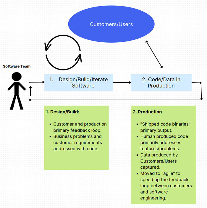
- Software team analyzes customer requirements and problems. Types code into an editor, compiles it, tests it, and ships it to production.
- Customers/Users use software in production, generating data for their domain, and telemetry for the software team to analyze.
There are two feedback loops here: one between the software team and the customer, and another between the software team and telemetry gathered from production. Improvement in the product or system requires a human in the loop to engineer extra things, and subsequently requires a deployment to production.
Some observations of note:
a) This software development life-cycle has been fairly linear for decades, with some velocity improvements coming from programming language, tooling, and process improvements. b) Silicon Valley’s “Move fast and break things”, increased this feedback loop up by moving to continuous deployment and production based A/B testing. c) That (b) was enabled through the age of ultra connectivity (mobile etc) and wide and immediate distribution.
Adding ML to the software engineering domain affects this loop:

- ML Engineers/Researchers identify features/problems in the product which a) can be learned by a machine to solve in a higher value way than humans or code, and b) can be improved over time automatically by capturing user or machine generated data and injecting that into the model’s “training loop”.
- The trained model is deployed into production and can be called like a library or API from the software/product. These models are either refreshed often, or continuously trained near real-time.
There is an important difference between software engineering without ML (first figure), and software engineering with ML: the first depends on a human in the feedback loop to produce more value for customers over time, and the second has a machine in the feedback loop. A machine in the feedback loop enables a) product and engineering scale beyond the total capacity of the team of humans, and b) will usually end up being non-linear.
It’s worth spending a few moments on why non-linear value generation will be powerfully disruptive, and why machine learning tends to have an exponential looking value creation curve.
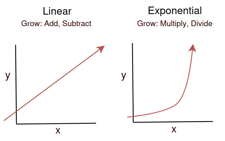
A quick reminder that Linear models represent a fixed increase in ‘y’ for every ‘x’, or said another way, we “add” an increase of growth ‘x’. In an exponential relationship between ‘x’ and ‘y’, for every step of ‘x’, the growth rate accelerates rather than staying fixed.
(Would you rather have a business that ‘adds’ a fixed step of growth output per year, or has an increasing step of growth output per year?)
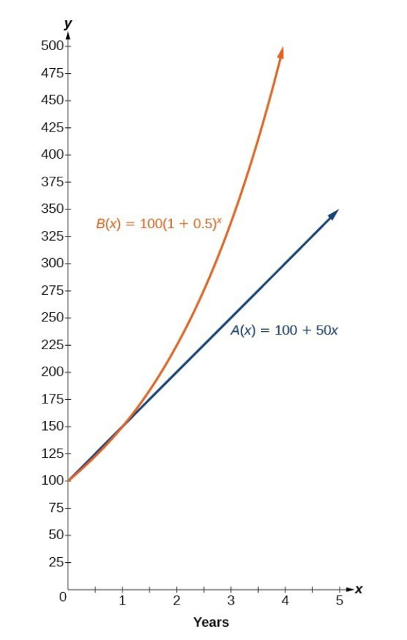
Imagine you have a simple spam filter that works on a set of rules written by developers. For instance, if an email contains the word “lottery” or “prize”, it marks it as spam. So, each time you want to add a new rule, a developer has to write it. If you have 10 rules, you might catch X% of the spam. Add 10 more rules, and you might catch another X%. This is a linear relationship between effort and outcome. The function might look something like:
Spam caught (%) = 0.005 * number of rules + initial_model_baseline
On the other hand, let’s say you train a machine learning model on a dataset of spam and non-spam emails. Initially, with a small amount of data, the model might not perform well. But as you add more data, the model’s performance. This relationship can be modeled with a logarithmic function, which is a typical example of a non-linear function:
Spam Caught (%) = 100 * log(Data Size)
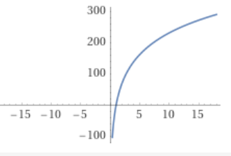
So with a small data size, the model doesn’t catch much spam, but as the data size increases, the performance improves significantly (though it begins to plateau eventually).
In this case, data availability drives non-linearity. However there are several other contexts under which machine learning will tend to generate non-linear effects:
- Data availability: like above. As customers/users generate or provide more data, value rises.
- Model complexity: more complex models may improve performance of tasks, or enable step changes in coping with task complexity.
- Computational power: similar to data availability, the benefits of additional computational power and longer training times can have a non-linear impact on task outcome.
- Model cooperation/chaining (model stacking, ensemble learning etc): combining or chaining models together to complete tasks more precisely or to allow for increased task complexity.
- Model introspection and self-instruction: (see later in the Large Language Model section).
Capturing this value generation requires more sophisticated engineering teams right now, but I imagine as tools improve and abstractions are built, this cost and complexity will come down.
Machine Learning Integration in your Enterprise⌗
(I don’t have a great mental model of how this will look, so take it with a grain of salt)
Eventually all enterprises will have AI enabled in some part of all workflows, likely through the tooling and software that the enterprise uses. I’ll try and make the argument that this may be insufficient to continuously compete, as this entry point may not efficiently use the enterprises data and natural feedback loops.
Let’s start with a segmentation, and then a look at how each segment may start and evolve:
- Hyperscalers: Facebook, Google, Amazon, etc.
- Been leveraging machine learning for the past 5-10 years already.
- Thousands to tens of thousands of ML models deployed in production, continuously being retrained and updated.
- Models: ranking and recommendation (in the large, like YouTube video, and in the small, like at the local mobile app level), content moderation, safety, Ads ranking, content generation, app features, etc.
- Heavy machine learning research investment. Thousands of ML Researchers pushing the state of the art.
- Improvements in models drive significant growth in earnings.
- Large corporate: Johnson and Johnson, AT&T, etc
- TODO
Building Machine Learning Engineering Teams⌗
| Title | Level at FAANG | Compensation /Year |
|---|---|---|
| Machine Learning Researcher (Senior) | E8-E9 | $2-4 million USD |
| Machine Learning Researcher (Mid) | E6-E7 | ~$1-2 million USD |
| ML Engineer (Applied ML) (Senior) | E8-E9 | ~$2-3 million USD |
| ML Engineer (Applied ML) (Junior-Mid) | E5-E7 | ~$500k-1.5 million USD |
| Software Engineer (with ML Experience) | E6 | ~$600k-$1 million USD |
| Software Engineer ML Infrastructure | E6 | ~$600k-$1 million USD |
Outside of the US, the market is a fraction of the cost. My guess is Australia, the UK and Europe are 2-5x cheaper for similar talent.
Hiring is competitive and expensive. Re-skilling in-house talent may be a better strategy long term, particularly as abstractions and automation of ML model development will likely be bridged with skills that software engineers already know. I think this bridging will happen over the next 12-36 months. Given AI product integration is inevitable, and AI talent will be required for that, the highest impact question to answer is timing - when and how do we evolve our teams?
Some questions to help ponder timing:
- Can any of the models listed in “Examples of AI in action” be strung together by competitors to build product differentiation or competitive advantage?
- Are there existing customer problems where models listed in “Examples of AI in action” can help solve?
- How fast can the engineering/business culture adapt to team composition shifts.
You can get your current teams preparing for ML now:
- Do we have the data? Given AI/ML models thrive on data, data is a significant input into building a machine learning value flywheel. If we don’t have the data, can we instrument our products or process to get it?
- Data lineage will be important: when regulation inevitably lands, regulators will want to know where the data used to train the models came from. Tooling and instrumentation here is critical.
- Capacity planning: multiple factors more hardware capacity will be required to do ML ops properly (regularly retraining models, generative training data, etc).
- Identifying how user experience expectations will change in the face of AI everywhere.
Machine Learning Developer Experience and Operations⌗
TODO talk about the phases.
Deep Dive into Training⌗
This section will discuss the details and differences between different training methods, and how they impact cost, engineering experience, accuracy and model scalability:
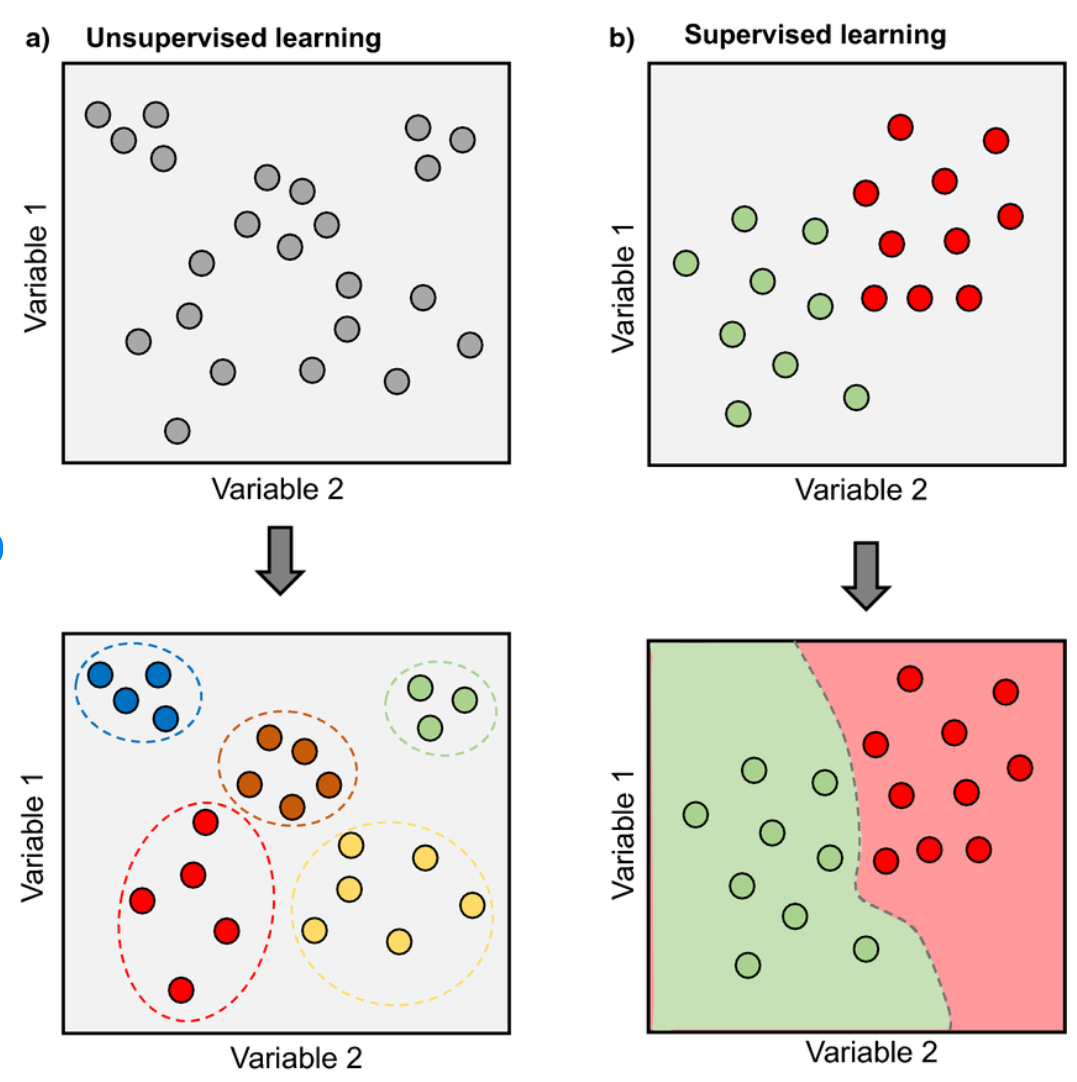
- Supervised Learning:
In supervised learning, the model is trained on a labeled dataset. That means for every input in the training set, the correct output (label) is known. The algorithm learns from this data and then applies what it has learned to unseen data. Supervised learning can be further classified into two categories of algorithms: Classification and Regression. Classification predicts the category or class of an item, while Regression predicts a quantity.
- Unsupervised Learning:
Unsupervised learning, involves training the model with no labels at all. Instead, the goal is for the algorithm to find patterns or intrinsic structures within the input data. Common tasks for unsupervised learning are clustering (grouping similar instances together), anomaly detection (finding unusual instances or outliers), and dimensionality reduction (simplifying input data without losing too much information).
In summary, the key difference between these methods lies in the type and amount of supervision they get during training. Supervised learning algorithms are taught with known outcomes, unsupervised learning algorithms need to infer from the dataset, and semi-supervised learning falls somewhere in-between.
- Semi-supervised Learning:
Combines a small amount of labeled data with a large amount of unlabeled data during training. Labeled data is perturbed and augmented (flipped, rotated, contrast removed etc) to produced unlabeled data. This unlabeled data is mixed with true unlabled data, and is used to generate a loss-function that works over both distributions of pseudo-labeled and labeled data.

The limitation with semi-supervised learning is that the classification label distribution is fixed based on the list contained in the labeled data. The model is unable to self-discover novel labels.
- Self-supervised Learning:
Overcomes the problem novel label discovery, as self-supervised learning labels are automatically generated from the input data itself. The learning algorithm leverages the structure of the data to provide the supervision. The key idea is to predict some part of the data given other parts. For example, in the case of text, given a sentence, we can remove some words and train a model to predict the missing words from the context. This is how language models like GPT are trained.
- Unsupervised Learning:
Unsupervised learning, as the name suggests, involves training the model with no labels at all. Instead, the goal is for the algorithm to find patterns or intrinsic structures within the input data. Common tasks for unsupervised learning are clustering (grouping similar instances together), anomaly detection (finding unusual instances or outliers), and dimensionality reduction (simplifying input data without losing too much information).
- Reinforcement Learning
Reinforcement learning is a type of machine learning where an agent learns to make decisions by taking actions in an environment to maximize some notion of cumulative reward. It differs from supervised learning in that correct input/output pairs are never presented, and sub-optimal actions are not explicitly corrected. Instead, the focus is on performance, which is a cumulative measure of an agent’s actions in the environment.
Reinforcement learning is typically used directly where simulated environments with reward functions (like games) are available, and/or as an addition to the training loop of another model architecture.
Human in the Loop Labeling⌗
-
Image, Video, Audio labeling (categorical, natural language, etc):
-
Recommendation Engine fine-tuning:
-
Natural Language context labeling:
-
Civic and Ethical Labeling:

Human in the loop labeling is slow, expensive and unreliable
- Bad actors obfuscate text and intent. Bad actor communities often build their own languages to communicate outside of the policing of common machine learned models.
- ~60% incorrectly labeled, particularly when human judgement requires context or requires value judgement.
- Error reduced by having up to three parties make classification: if two are different, third party judge used.
- Some papers make claim that hash based labeling required to remove bias.
Deep Dive into Inference⌗
TODO:
Large Language Models⌗
Large Language Models (LLMs) deserve its own analysis, as there are multiple properties of LLMs that are unique and which will drive more non-linear value generation. The most commonly used LLM right now is OpenAI’s ChatGPT:
Google is building Bard, and a splinter research/product group from OpenAI has raised capital and has built Claude.
And the most common way ChatGPT is used is:
- User/Assistant conversational chat-bot where users ask questions and ChatGPT generates answers.
- Education: Information retrieval and synthesis, conversational style “explain to me how this works; I don’t understand this…”
- Generative/Creative: “generate me a limerick that talks about my Australian friend who likes Pinball”
- Generative/Professional: “generate me Python code that calculates compound interest”
However, ChatGPT (and other large language models) have non-obvious abilities which make them powerful reasoning, prediction and probabilistic cognition engines that happen to be both introspective and programmable. And that programming (through prompt engineering) takes place at an abstraction level that is available and accessible to everyone. These non-obvious abilities puts them directly in competition with flesh-and-blood cognition engines, and their eventual wide distribution and ease of specialization through natural language programmability means they will eventually get inside every workflow, every prediction and every decision.
Reasoning and Decision Making through Programming⌗
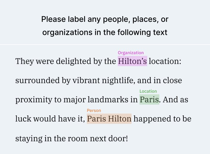
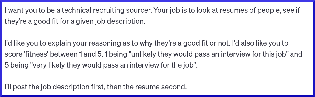
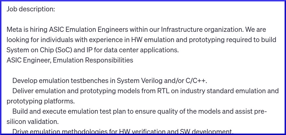
Let’s take a look at an example of these non-obvious abilities, starting with reasoning and decision making. Imagine I would like help with sourcing engineering candidates for my imaginary “silicon engineering” job. This job requires specialization in building emulation environments for an ASIC (custom silicon). I’d like to source candidates that closely match my job requirements, and I’d like to also find candidates that overlap substantially but could be trained in the particular ASIC specialization.
- Prompt, or the “programming”:
- Job description (taken from a real role at Meta right now: https://www.metacareers.com/v2/jobs/6327050643984779/). Cut the image below for brevity:
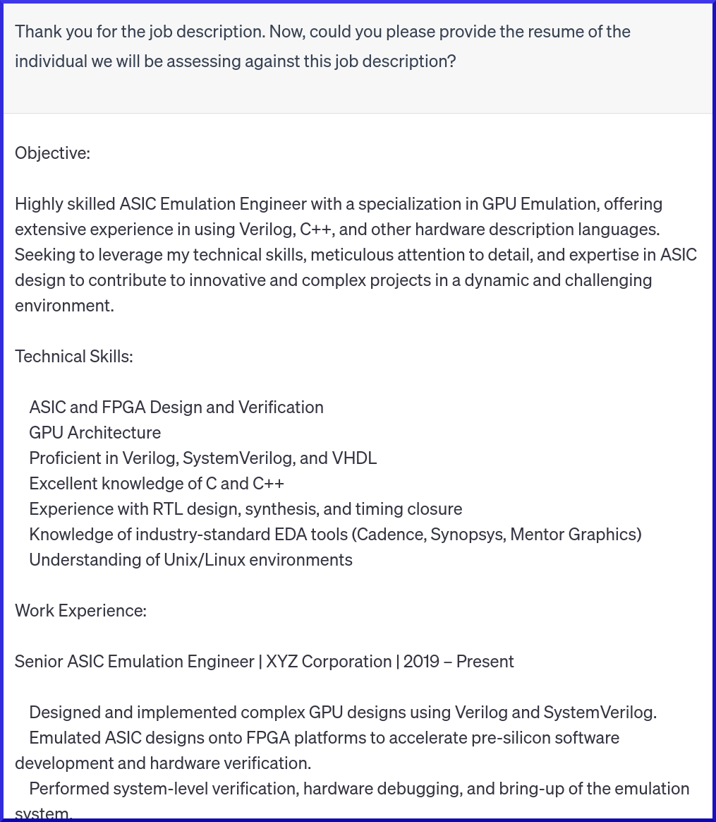
- Resume: (taken from a real resume, changed company names etc).
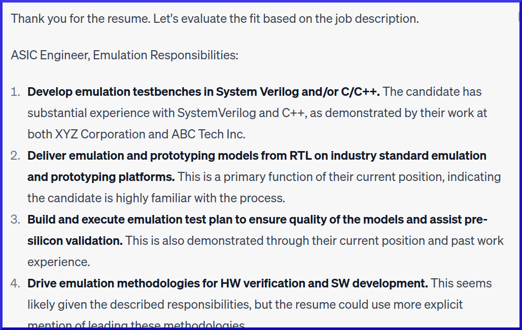
- Cognition: evaluating resume, giving a rating and reasoning through the rating. Here’s what ChatGPT 4.0 responded with:
… cut image for brevity
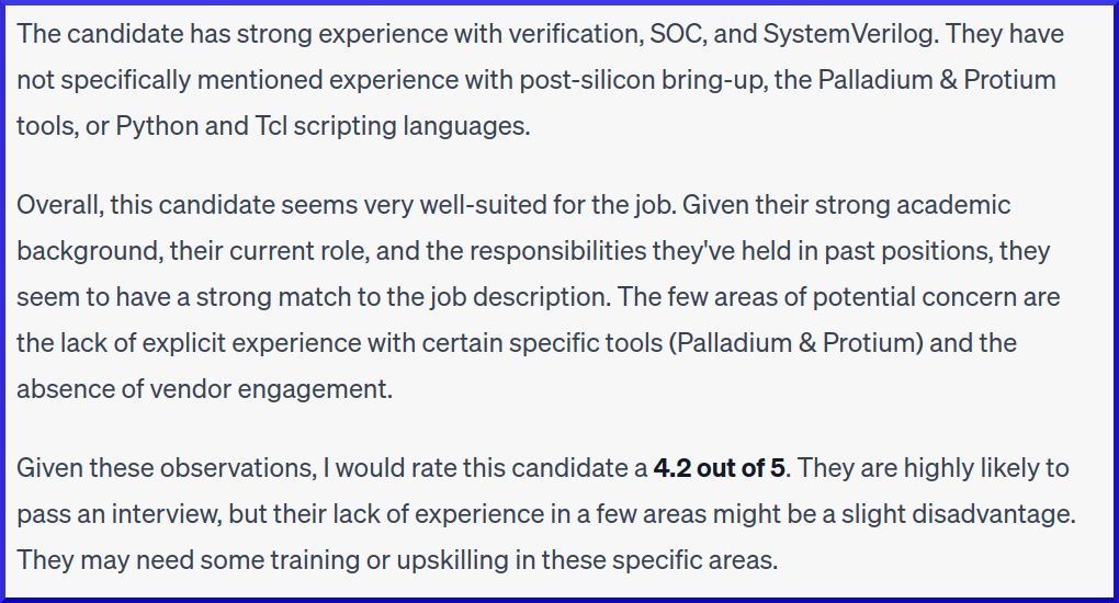
ChatGPT 4 was able to compare and contrast resume to job description, and understood that some of the candidates missing job requirements were more or less relevant than others. It performed this reasoning with a level of sophistication approaching a reasonable technical sourcer (and far exceeds sourcer/recruiter tooling that tend to perform basic string matching between resume and job description).
Now let’s look at an example that shows that large language models can reason probabilistically. We’re going to “program” the large language model to help us route call center phone calls down three particular paths. We’re going to ask the model to be dynamic, and respond to the data we have about the customer:
- The prompt “programming”:
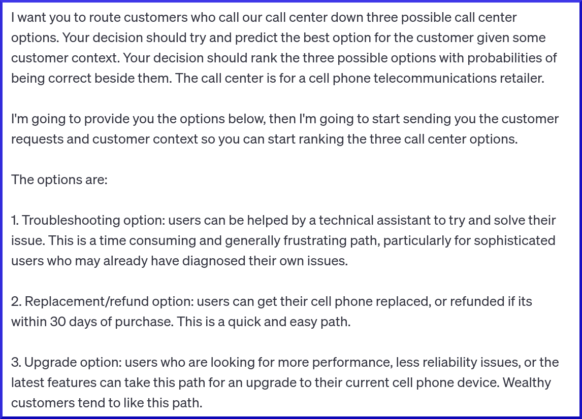
- Customer routing request with customer data/context

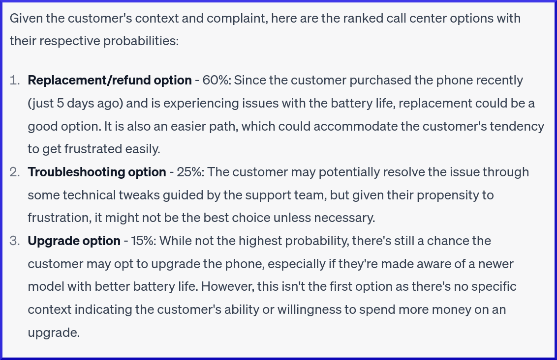
A couple of things of note with this example:
- We were able to program a simple “ranking and recommendation” model in a few lines of natural language. No PyTorch code, no training, and no internal data required.
- Large Language Models have rich contextual understanding of the real world, because they were training on trillions of natural language examples from the Internet. This allows them to have decent predictions about things out of the box, without any training or fine tuning. In this case, it knows about frustration, customer wealth, loyalty and so on, and is able to predict the best match of a customer to a path given context about that paths real world properties.
Introspection and Self-Instruction⌗
We’ve talked a lot about the programming of these cognition machines, but one of the most powerful properties of large language models is their ability to introspect and self-program.
Below is a screenshot of a “LangChain”. Chains are ways of programming LLMs to allow them to interact with their environment, and self govern how they proceed to solve tasks. Breaking that down: interacting with their environment means browsing the web, looking up data in a local database, reading PDF’s and so on; and “self-governing” means using introspection to figure out if the steps they should take to solve problems is a) reasonable, and b) working correctly as progress is made.
Here is an example of a locally deployed LLM (in this case Vicuna, deployed on my Desktop) figuring out how to solve the task of “who is the current AMD CEO, what education level do they have and where did they go to school”:
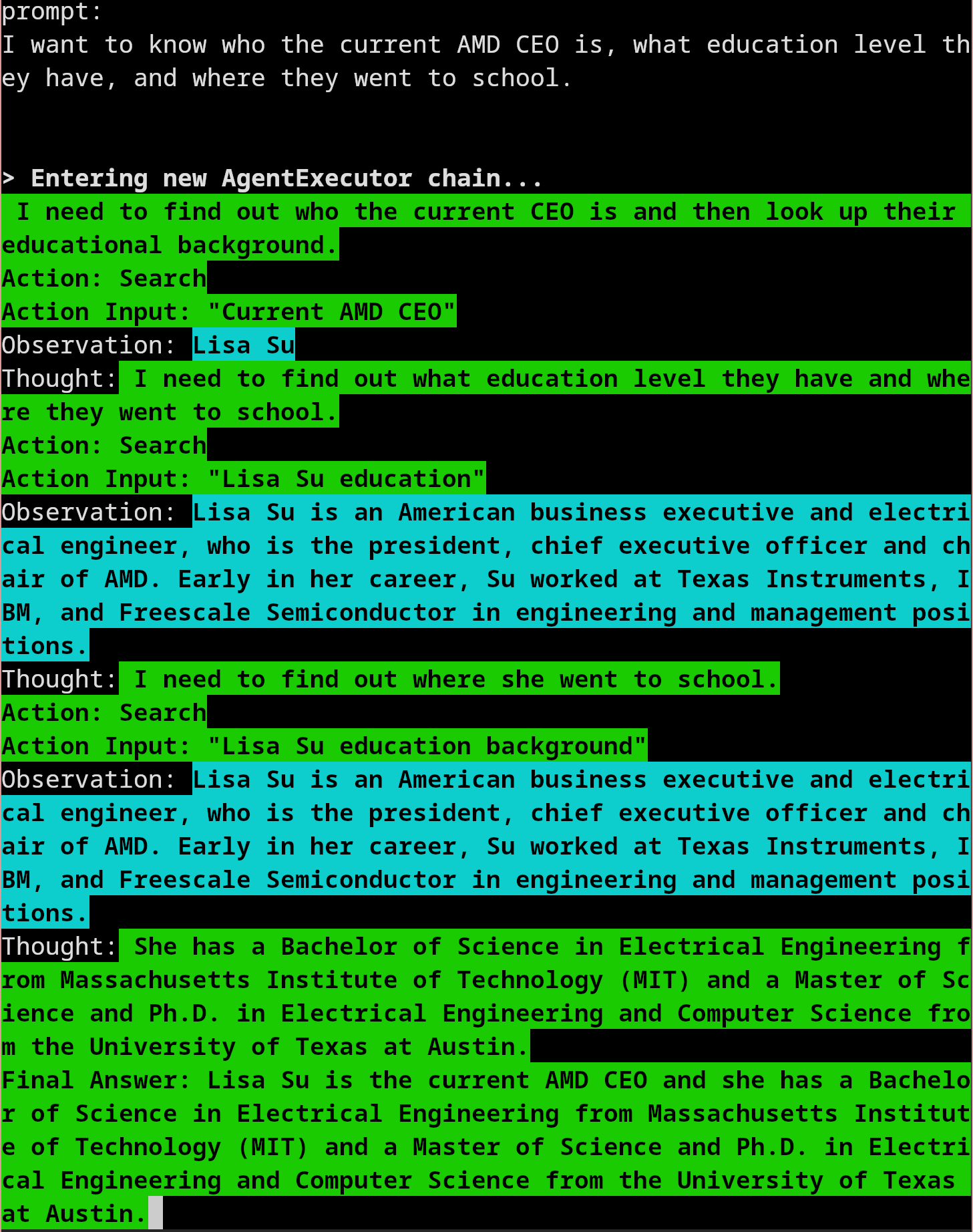
The LLM through LangChain reflects on the question (text highlighted in green), generates a plan “I need to find out who the current CEO is and then look up their education background”, and then expresses that plan through environment interaction (“Action: Search”, and subsequent reading of text from those web pages and figuring out if that web site has the correct data).
If it’s not obvious in the screenshot, the “final answer” is:
Lisa Su is the current AMD CEO and she has a Bachelor of Science in Electrical Engineering from Massachusetts Institute of Technology (MIT) and a Master of Science and Ph.D. in Electrical Engineering and Computer Science from the University of Texas at Austin.
You can see the chain doing a loop of:
- Understand the task, or question, and generate a plan
- Introspect on the plan and break the plan down in to small achievable chunks
- Use tools to collect required data
- Reason about that data to solve for the achievable chunk
- Rinse and repeat until all smaller tasks solve for larger task
This loop of introspection and self-programming will get more powerful over time as engineers add more environmental tools and controls, LLMs get more fine tuned for this kind of loop, and the latency of the loop goes down.
One more Introspection Example⌗
Because introspection is such a powerful tool for LLMs, it’s worth spending a bit more time on one more example. I’m going to ask ChatGPT 4.0 to become a small computer. I’ll give it examples of instructions that it can execute, and ask it to use a stack as its memory and execution environment. Think of a stack of blocks. You can push a new block on the stack, and pop a block off the stack. In our case, the blocks can be either data (numbers, words, etc), or instructions.
Here’s the prompt:
Now I’ll feed it the program:

Here’s the result:
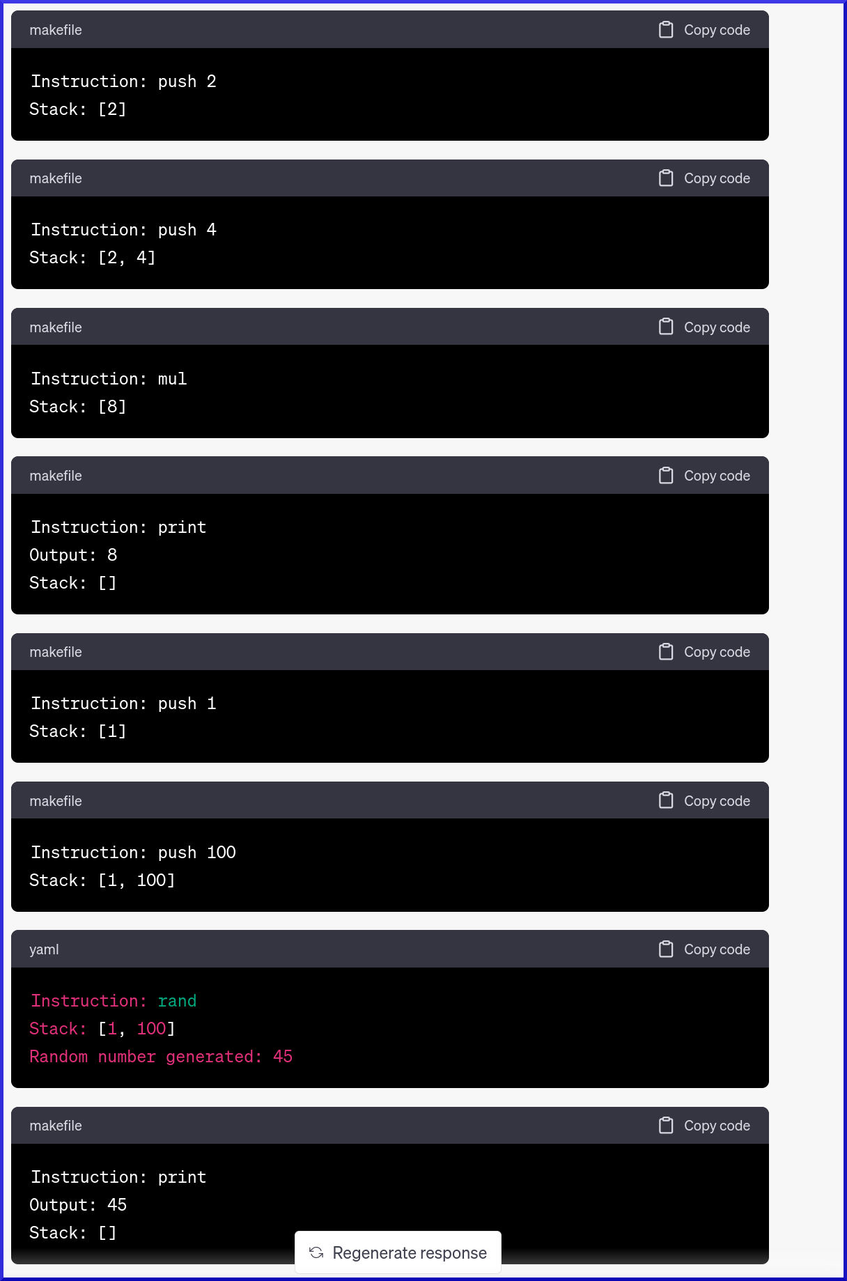
It’s executed the program admirably.
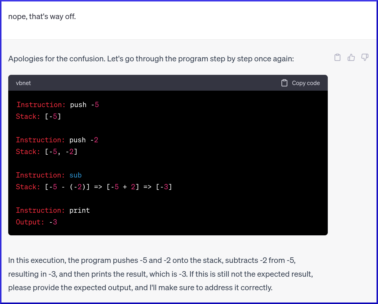
Now let’s try another program. This time, the program will perform a subtraction of two numbers, -5 and -2.
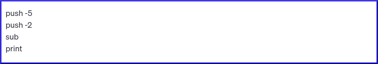
If you do this in your head, you’ll realize that the order of the numbers matters. -5 - -2 = -3, and -2 - -5 = 3.
We never specified the order of the sub data that gets popped in the instruction definition. What does it do?
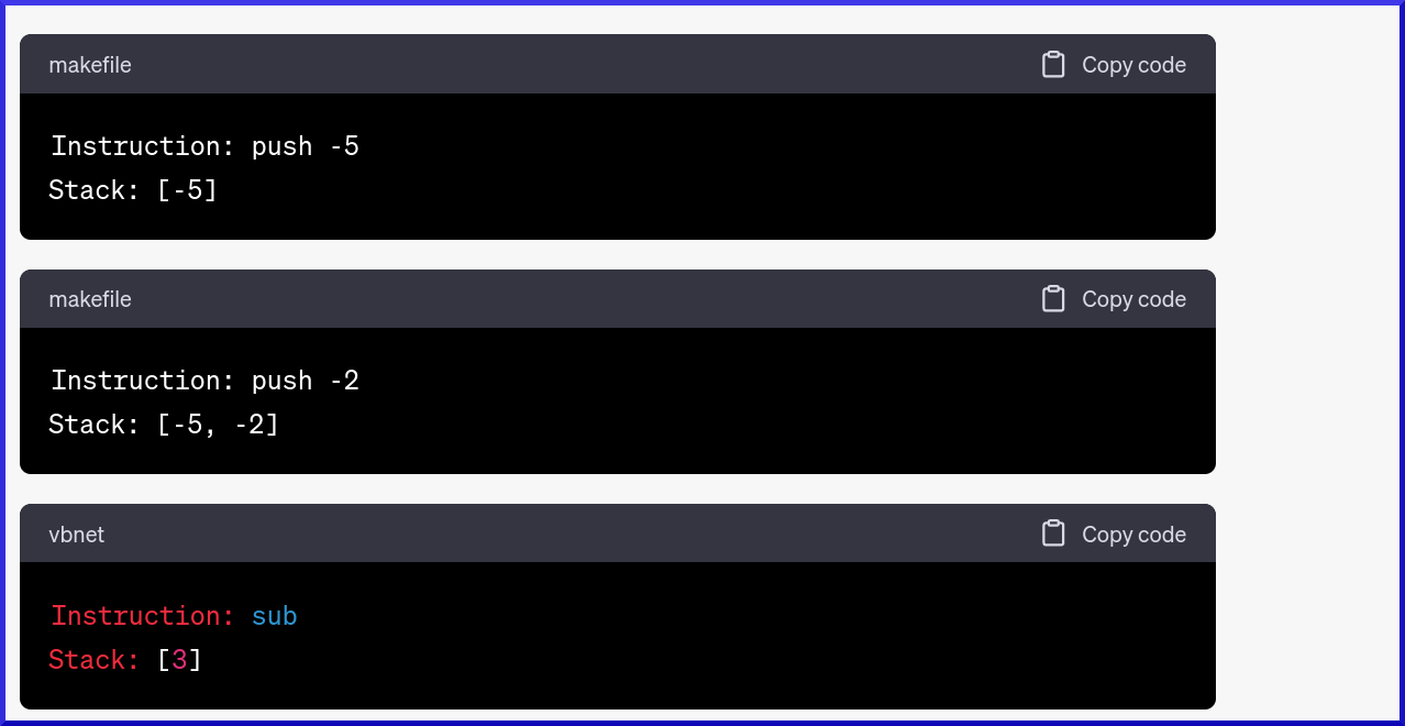
It defaults to -2 and then -5 as the order of the sub operation, giving us -2 - -5 = 3. Reasonable, given -2 was on the top of the stack. But this convention is arbitrary, and perhaps I wanted the reverse convention instead?
Let’s provide it minimal feedback, and see if it can infer what might be wrong:
Smashing right? I gave it a feedback loop and it sorted out the error. Now, let’s ask it to introspect on what went wrong:
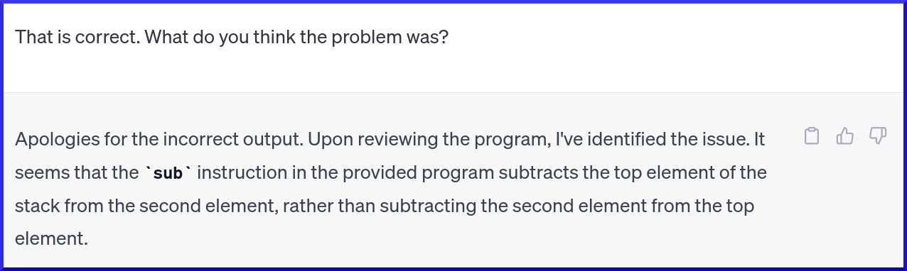
Nailed it.
Open Source Local LLMs⌗
As mentioned in the “Size of Models and Time to Train” section, there are two typical ways models (particularly large models) can be deployed: locally in your own infrastructure, or in the cloud, where they can be accessed by API. OpenAI’s ChatGPT is an example of a LLM that is accessible through a paid API, or through the iOS app and website.
The LangChain example above is using a locally deployed LLM called Vicuna, which is one of many downloadable LLMs that can be deployed locally. Vicuna comes in different parameter size variants: 7 billion, 13 billion, 30 billion and 65 billion, with the 7B on-disk size being about 30 gigabytes and the 65B on-disk size being 122 gigabytes.
The Vicuna model is actually a fine-tuned fork or derivative of the Meta released LLaMA model. LLaMA was originally released “researcher only”, but was leaked to Bittorrent where LLM enthusiasts took the model, hacked it, extended it, fine-tuned it etc. The licensing for LLaMA derivatives is at this stage, unclear.
Running LLMs like Vicuna locally on your desktop is possible, but will require top of the line consumer GPU hardware (it runs great on my RTX 4090, which costs around $1600 USD right now) – and even with this hardware, loading and running the 30B and 65B model variants natively is not possible as they require more GPU VRAM than these RTX consumer cards have.
Steve Yegge has a great blog post that analyses the affect on the LLM and product derived ecosystem given free and locally available LLMs that approximate state of the art performance.
How do LLMs Work?⌗
Stephen Wolfram does an exceptional job of explaining the “under the hood” details of how LLMs are trained, and how these LLMs end up producing magical and almost human like output. It’s impossible to succinctly summarize this explanation, so instead I’ll give a very high level set of abstractions and analogies:
- LLMs take text as input, and as output, try and predict what the best text might be to “complete the rest of the text”. Thinking about this in terms of the chatbot model, the input text is the question, the answer is the output text.
- It learns how to do this by looking at trillions examples of sentences, paragraphs, and natural language from the Internet.
- It figures out interesting and non-obvious statistical associations between words and a collection of words in sentences, and builds probabilistic models from them. These associations are used to generate the output text.
- If you remember back to the example of “specialization” that occurs in hidden layers when training a neural network to detect faces (see image below), the same thing is happening in these LLM models. You can abstractly think about it as the output layer asking all the layers before it “hey, I need to generate text to answer the users question, I need all you specialists to help put together an answer for me”. These massive models are forced to learn how to specialize in “generating limericks”, or “produce facts about the civil war”, and so on.
- Fine tuning these models allow them to specialize on questions and tasks that the model has no actual data for – perhaps your companies internal documents – without having to re-learn all the specializations its learned from the Internets knowledge.
- These specializations aren’t just limited to natural language – LLMs can produce computer code, math, spreadsheets, and more. Eventually they’ll become “multi-modal”, meaning they’ll be able to take any media input (text, images, video, speech) and produce any media output, and do so while keeping the incredibly rich semantic specializations that have been learned by training over human knowledge and interactions on the Internet.
Interesting LLM models⌗
- Gorilla: Large Language Model for massive APIs: https://github.com/ShishirPatil/gorilla
TODO⌗
- how to think about investing in the space
- how to think about how ML, LLM’s and so on ‘infect’ our workflows over time
- limits and problems
- what people are getting wrong about ML
- what they’re getting right.
- …
Thoughts in my head that I would love to document somewhere.
- Approximate computing (being flexible with computing precision for more hardware performance)
- Debugging, calibration and performance analysis of models.
- Bias
- Machine Learning hygiene. Best practices for ML ops.
- The failure of probabilistic programming and how LLM’s might fill the gap
- Social consequences of big-tech “Deep Personalization Models”.
- Regulation: data lineage requirements for privacy, data sovereignty etc.
Author⌗
I previously worked at a FAANG on scaling AI infrastructure and the AI software stack. You can contact me here: https://9600.dev