Machine Learning Notes for Developers
Machine Learning systems notes. Some ‘ML’ math at the start, hardware stuff in the middle, training/inference and optimizations at the back. LLMs TBD.
Linear Models⌗
Simplest linear model:
$$ y = mx + b $$ $$ y = 2x + 3 $$
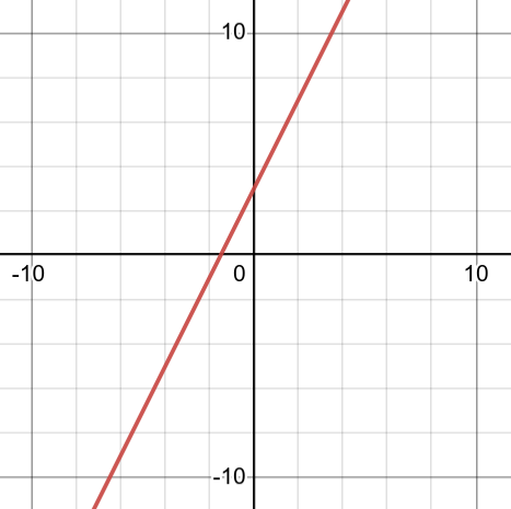
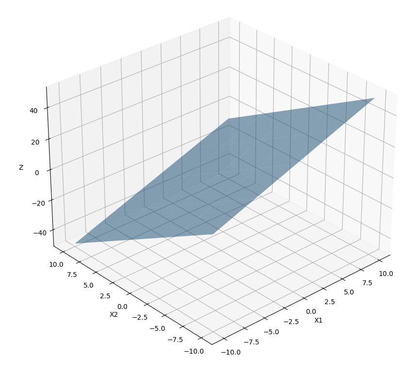
Where ‘x’ is the input, and ’m’ is the parameter in the context of machine learning. A multivariable linear function generates a plane. In this instance, a plane in three dimensional space:
$$ z = m_1x_1 + m_2x_2 + \dots + m_nx_n + b $$
Example:
$$ z=2x_1−3x_2+1 $$
 Defining a linear function in terms of multiple variables:
$$ y=m_1x_1+m_2x_2+…+m_nx_n+b $$
Parameters⌗
A parameter is a quantity that influences the output or behavior of a mathematical object but is viewed as being held constant. Parameters are closely related to variables, and the difference is sometimes just a matter of perspective. Variables are viewed as changing while parameters typically either don’t change or change more slowly. In some contexts, one can imagine performing multiple experiments, where the variables are changing through each experiment, but the parameters are held fixed during each experiment and only change between experiments.
One place parameters appear is within functions. For example, a function might a generic quadratic function as
$$ f(x)=ax^2+bx+c $$
Here, the variable x is regarded as the input to the function. The symbols a, b, and c are parameters that determine the behavior of the function f. For each value of the parameters, we get a different function. The influence of parameters on a function is captured by the metaphor of dials on a function machine.
Messing with lines⌗
Adding lines:
$f(x) = 3x - 1$
and
$g(x) = -x + 2$
$h(x) = f(x) + g(x)$
$h(x) = (3x-1) + (-x + 2)$
$h(x) = 2x + 1$
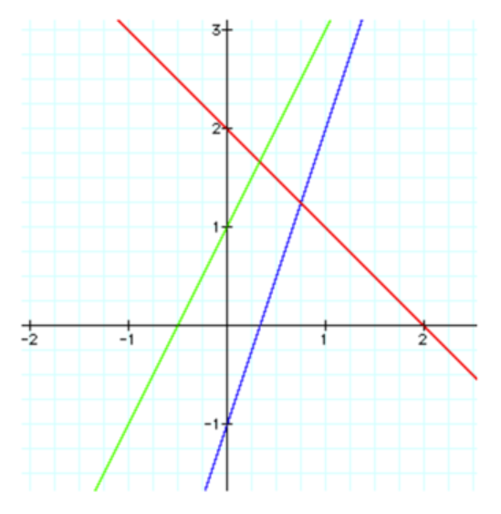
where $f(x)$ is blue, $g(x)$ is red and $h(x)$ is green.
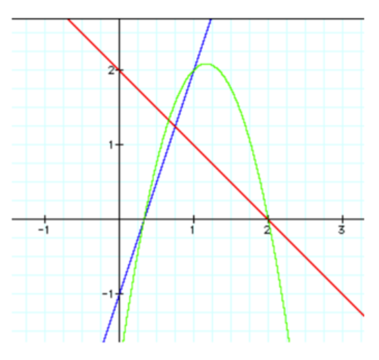
Multiplying two linear functions will always be quadratic (parabola), because the degree of ‘x’ will always increase to 2.
$h(x) = f(x) \cdot g(x)$
$h(x) = (3x - 1) \cdot (-x + 2)$
$h(x) = -3x^2 + 7x - 2$
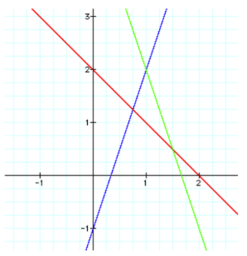
Composition of linear functions:
$h(x) = f(g(x))$
$h(x) = 3(-x + 2) - 1$
$h(x) = -3x+5$
Matrices⌗
An exceptional article explaining matrix math is here.
Matrix multiplication is about information flow, converting data to code and back
Before we look at this analogy, remember that order matters in matrix multiplication: $ A _ B $ does not equal $ B _ A $ because the size of the matrices can be different and when swapped, the shape of the output will change too.
$$ \left[ \begin{array}{cc} 1 & 2 & 3 \\ 4 & 5 & 6 \\ \end{array} \right] \cdot \left[ \begin{array}{c} 7 \\ 8 \\ 9 \\ \end{array} \right] $$
2 x 3 and 3 x 1 (last and first terms are the same, this multiplication is possible)
$$ \left[ \begin{array}{ccc} (1 \cdot 7) + (2 \cdot 8) + (3 \cdot 9) \\ (4 \cdot 7) + (5 \cdot 8) + (6 \cdot 9) \\ \end{array} \right]=\left[ \begin{array}{c} 50 \\ 122 \\ \end{array} \right] $$
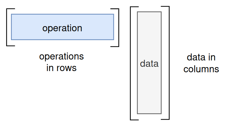
A matrix can be seen as a collection of data points or as a collection of functions. Depending on the context and desired outcome, we can interpret the matrix in different ways.
iFor example, if we interpret a matrix as a collection of data points, we can think of matrix multiplication as performing calculations on that data. On the other hand, if we interpret the matrix as a collection of functions, we can think of matrix multiplication as composing those functions.
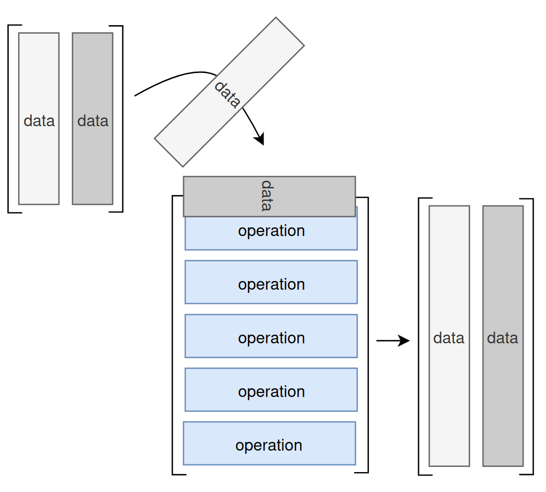
An example of this analogy follows:
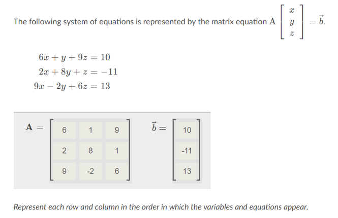
A major application of matrices is to represent linear transformations (i.e. f(x) = 4x. e.g. rotation of vectors in three-dimensional space is a linear transformation, which can be represented by a rotation matrix.
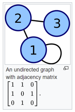
Another application is for graph theory, where you can build an ‘adjacency matrix’ for a finite graph. It records which vertices of the graph are connected by an edge as seen below. For huge graphs (websites connected by hyperlinks etc), these matrices tend to be very sparse, so there are other matrix representations/algorithms? that can be used in network theory.
Links⌗
Because Linear Algebra, Calculus and Matrix math are used heavily in Machine Learning, it pays to pay attention to them:
- Numerical Linear Algebra - fast.ai
- How is calculus different from algebra
- Graphical understanding of partial derivatives
Neural Networks⌗
Leverage multiple linear models composed together to build a more complicated non-linear model. Non-linearity comes via two things: 1) the composition of multiple linear layers, and 2) activation functions.
Typical deep learning neural network:
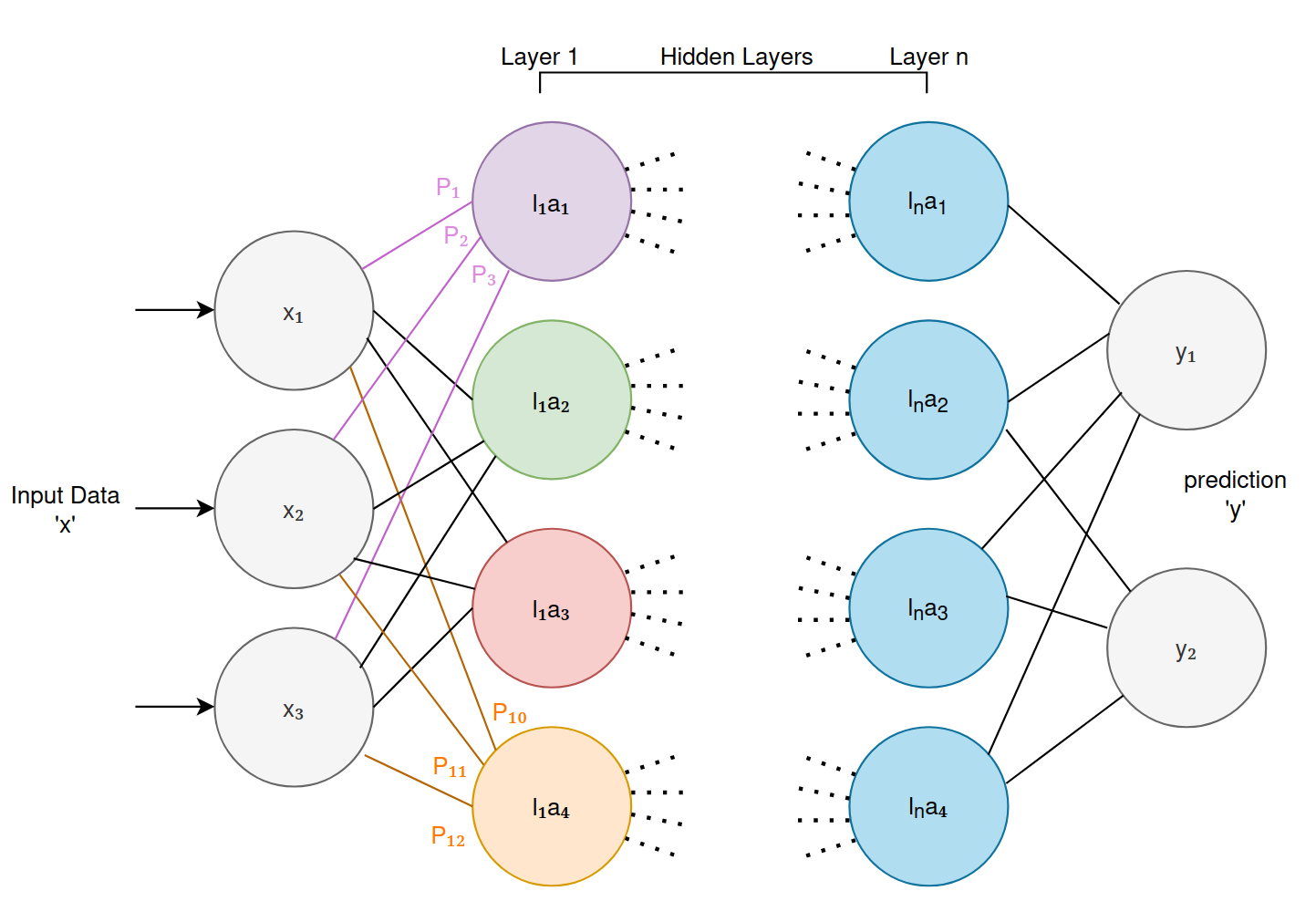
- Each of those colored circles are “neurons”.
- Each neuron receives “data” from any connections to other neurons it has to its left. The biological equivalent being “synapses”.
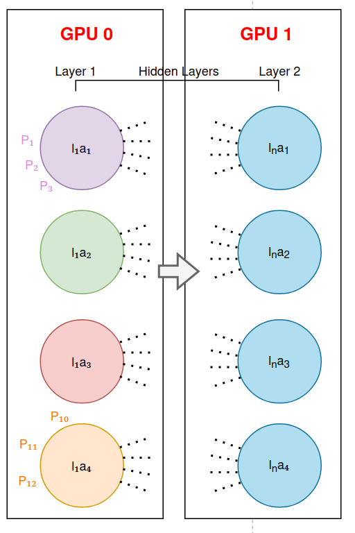
- Each of those data are multiplied by ‘parameters’ or ‘weights’ and then summed up. Essentially calculating the equation we saw above:
$$ l_na_z = P_1l_1a_1 + … + P_zl_na_z + b $$
Where ’l’ is the layer, and ‘a’ is the neuron, ‘b’ is the bias. Sometimes expressed as:
$$ b + \sum_{i=1}^{n} x_i w_i $$
An activation function is applied post-calculation:
$$ activation_function\left(b + \sum_{i=1}^{n} x_i w_i \right) $$
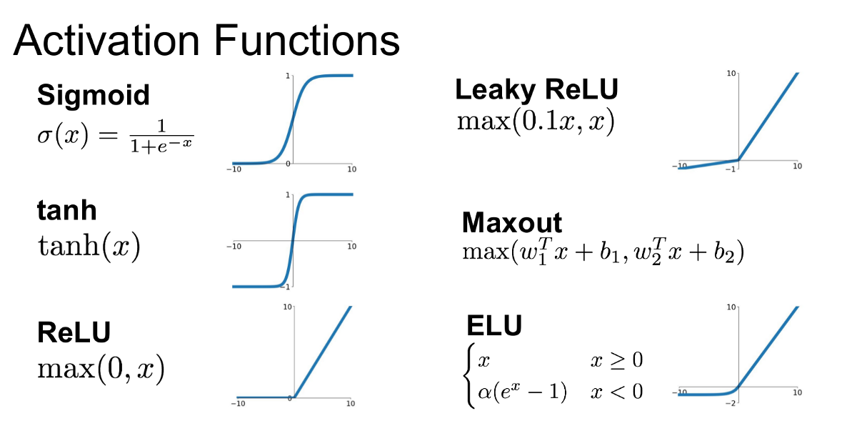
Picking an activation function is dependent on the type of convergence property you want your layer to have.
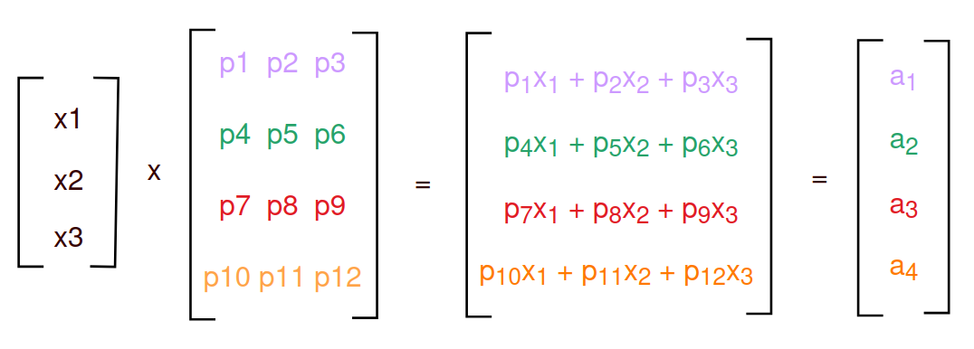
A useful property of a feed-forward neural network is that data passing through the network can be lowered down to matrix math (x1 -> x3 is the input data, and p1 -> are the weights for the first layer of four neurons in the example above):
The analogy of matricies being both data and functions applies to neural networks nicely - “data” from the input layer is applied to each of the neural nodes, which are essentially “functions” that are learned over time by the training loop.
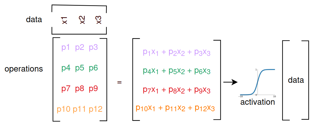
Activations are applied (generally on a per layer basis) to aggressively move forward capture of non-linearity in the model.
Each layer is producing “data” for the next layer of the network, which essentially is performing another transformation on that data for the next layer and so on. There are two useful mental models for what is actually going on here. In the small, the first mental model is that each layer/neuron is “signaling” to the next layer “hey, I’ve seen this before” for values that are positive, and “I’ve not seen this before” for values that are neutral/negative. The second, more abstract and likely more useful, is that each layer/neuron is specializing on a particular task, which is ultimately required for the next task in the pipeline. This is seen in the following visualization of a image recognition neural network:
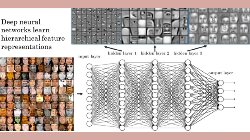
In this example, the first layer is learning contrast and edges, which is then used for the second layer to perform identification facial features, which is useful for the third layer which is putting together a represention of a full face. To perform the visualization, each layer output for a given piece of data has been transformed into “pixels” so we can see what it’s signaling as “yes, I’ve seen this before” (i.e. a bright or dark set of pixels) vs. “no, I’ve not seen this before”, which could look like a monotone blank square.
Weighted Sum⌗
This signaling from each neuron as “hey I’ve seen this before” is because the fundamental calculation each neuron is performing is called a “dot product” (or “weighted sum”, or “inner product”), essentially the equation we saw above:
$$ l_na_z = P_1l_1a_1 + … + P_zl_na_z + b $$
(although neurons also have bias, and activation - bias gives the neuron a little more room to maneuver)
If the equation results in zero, the vectors are perpendicular. If the result is positive, they’re similar, and negative dissimilar. The range is +- infinity, so we scale it to -1 to +1 by normalizing each vector before the np.dot call:
a = np.array([0.3, 0.4, 0.5])
b = np.array([0.3, 0.4, 0.5])

np.dot(a, b)
> 0.5

np.dot(a / np.linalg.norm(a), b / np.linalg.norm(b))
> 0.99999999999
With a normalized “weighted sum” a neuron can say “1.0, the input matches my weights perfectly”. This matches what we’re seeing in the visualization of the face recognition model above: you feed input data of a face to a given layer, and the neurons in that layer “light up” (go to 1.0) when they recognize the features they’ve been specialized to see.
Training⌗
Machine learning training involves using a large dataset to “teach” a model how to perform a specific task (like the example above of classifying faces), by adjusting the model’s internal parameters to minimize the error in its predictions over the course of training.
The psuedocode for the training loop looks like this:
- Initialize random weights for the model
- For each piece of data -> prediction pair (i.e. the data you’re inputting, and the correct answer for the given task), do:
- Push data through the model
- Compare the output of the model with the correct prediction
- Calculate the error (the difference between the models prediction and the answer)
- Backpropogate the error through the weights of the model
Back-propagation is the term given for the mathematics to calculate the change required in each of the model weights/parameters in order to reduce prediction error next time around. This is done by calculating the derivative of the error, i.e. the direction and slope of the current training output with respect to the correct prediction:
from quantinsti.com:
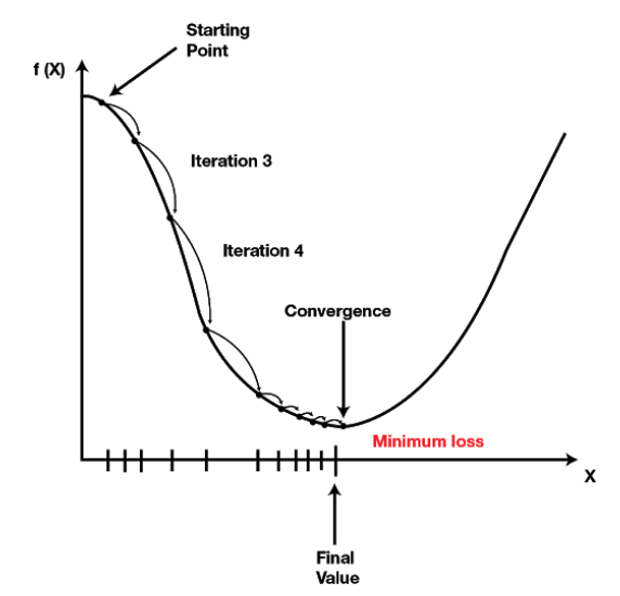
$f(X)$ is the plot of the error. The “starting point” is early in the training loop, the “final value” is the correct prediction. For each iteration of the training loop, calculate the error direction and slope by deriving the model prediction with respect to the correct value, and send that “direction and slope” backwards through each layers weights, nudging them in the correct direction.
The calculation of each weights movement and magnitude is done through the chain rule and partial derivatives, which is explained in detail here.
Inference⌗
Once the model has been trained (or ‘converged’, meaning training is not substantially improving its predictive performance), the model can be packaged and deployed for use. Inference is the term used to describe the act of pushing unknown data inputs through the network to get an output or prediction for use. There is no data/answer pair (the data for inference is generally out of sample, meaning it wasn’t seen during training), so there is no back-propagation pass.
Size and Scope of Neural Networks⌗
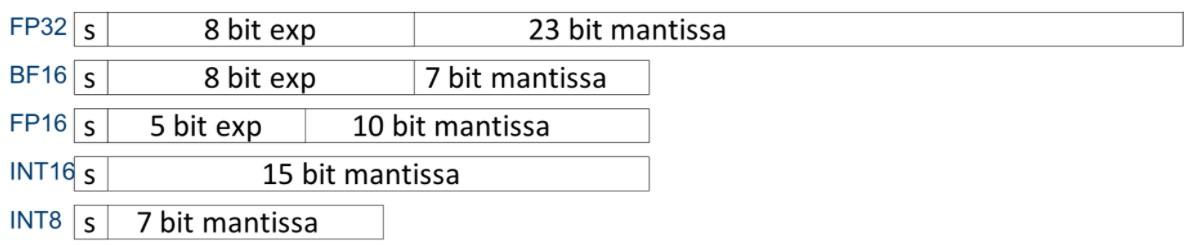
The following table shows the relative size of different types of deep learning networks. Weights during training are typically represented as either 16 bit floats (half precision) or 32 bit, so to calculate a rough order of memory required for training:
$\text{Parameter memory} = \text{Num}\space \text{of}\space \text{parameters}\space \times N\space \text{bytes}$
$\text{Activation memory} = \text{Num}\space \text{of}\space \text{activations}\space \times N\space \text{bytes}$
$\text{Gradient memory} = \text{Num}\space \text{of}\space \text{parameters}\space \times N\space \text{bytes}$
where $N$ is the precision used for training (2 for 16 bit training, 4 for 32 bit).
| Model | Training Time | Size | Compute |
|---|---|---|---|
| XOR | Milliseconds | 4 parameters | Laptop |
| Snake | Minutes | 12 parameters | Laptop |
| MNIST Digit Classification | Hours | 100-300 thousand | Laptop |
| ImageNet image classifier | 15-20 hours | 25-150 million | Desktop |
| YouTube Ranking and Recommendation | Weeks | Billions | Server Farm |
| Llama 2 Language Model | Months | 7-70 billion | Data Center |
| ChatGPT Language Model | Months | 100’s billions | Data Center |
The Llama 2 paper shows total time, power consumption and carbon emitted to train:
| Size | Time (GPU years) | GPU’s | GPU (W) | Power Consumed (MW) | Metric Tonnes CO2 |
|---|---|---|---|---|---|
| 7B | 21.3 | 2048 | 400W | 73 MW | 31.22 |
| 13B | 42.6 | 2048 | 400W | 147 MW | 153.90 |
| 70B | 199 | 2048 | 400W | 688 MW | 291.42 |
(as an aside, the Las Vegas power generation station produces 359 megawatts of natural gas powered electricity, reference)
Inference⌗
Given inference doesn’t require the backwards pass, the memory requirements are very different, just requiring space for parameters and input data:
$\text{Parameter memory} = \text{Num}\space \text{of}\space \text{parameters}\space \times N\space \text{bytes}$
The model can also be “shrunk” or “compressed” through quantization of model parameters. As the Hugging Face doc mentions: “Quantization is a technique to reduce the computational and memory costs of running inference by representing the weights and activation’s with low-precision data types like 8-bit integer (int8) instead of the usual 32-bit floating point (float32).”
An example of the process is detailed in this NVIDIA technical blog, but the basic premise is you’re looking at the distribution of neuron results, then using a smaller, less precise value to represent that distribution:
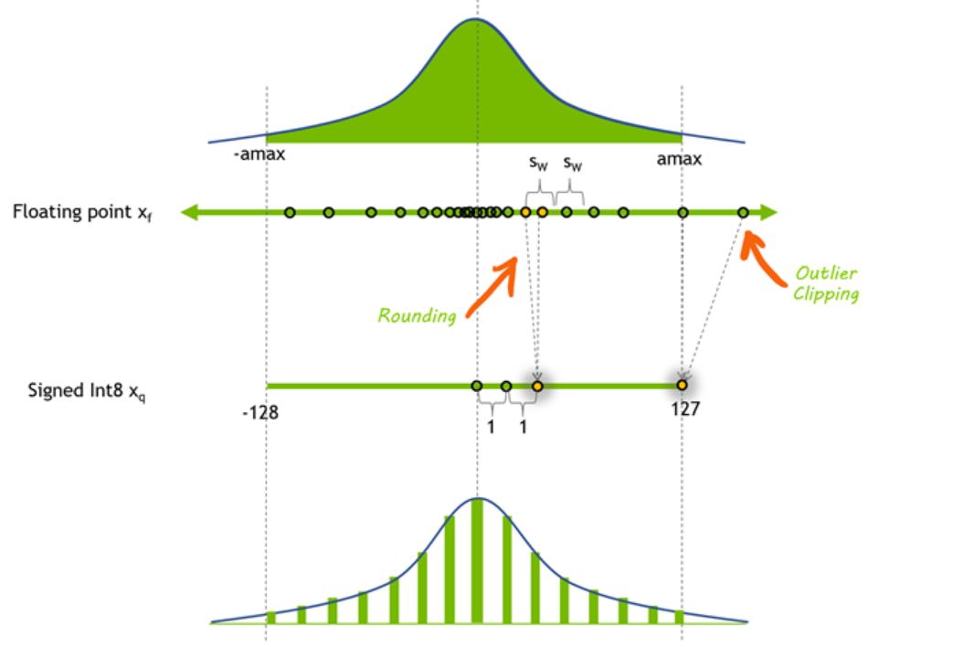
Shrinking from 32/16 bit to 8 or even 4 bit significantly improves the performance of inference (throughput and latency) at the expense of model accuracy. It also allows large models like Llama 2 to be shrunk and deployed on consumer grade video cards (ones with 12-24 GB of VRAM). This link has 2, 3, 4, 5, 6 and 8 bit quantized versions of Llama 2 13B, with the maximum memory required being ~14GB.
Both the forward pass (the prediction of the model, given data), and the backwards pass (the nudging of weights in the training loop given error) are perfectly suited to GPU acceleration, given most of it is matrix math, which GPU’s have specialized for years given 3D games use matrices to represent polygons (data), and transformations of polygons (functions, like rotation) in 3D space.
Neural Networks as Code⌗
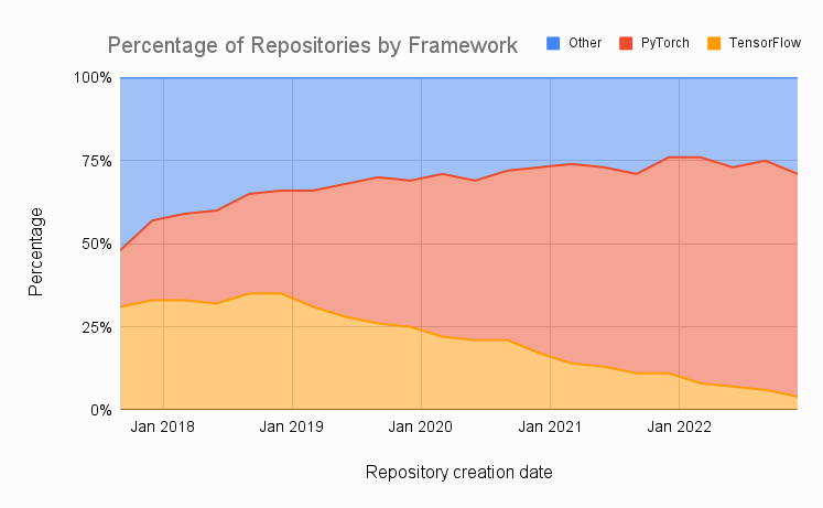
The Python based PyTorch framework is the clear winner right now in terms of researching and productionizing deep learning models:
Simple PyTorch example of learning the a model for XOR (eXclusive OR):
| A | B | A XOR B |
|---|---|---|
| 0 | 0 | 0 |
| 0 | 1 | 1 |
| 1 | 0 | 1 |
| 1 | 1 | 0 |
Imports and defining the data:
import torch
import torch.nn as nn
import torch.optim as optim

# Define the XOR dataset
X = torch.tensor([[0, 0], [0, 1], [1, 0], [1, 1]], dtype=torch.float32)
y = torch.tensor([[0], [1], [1], [0]], dtype=torch.float32)
Define the PyTorch Model: 2 inputs (A and B), one output (result):
# Define a simple neural network with one hidden layer
class XORNN(nn.Module):
    def __init__(self):
        super(XORNN, self).__init__()
        self.fc1 = nn.Linear(2, 2)  # Input layer with 2 neurons (for 2 input features)
        self.fc2 = nn.Linear(2, 1)  # Output layer with 1 neuron (for 1 output)
        self.relu = nn.ReLU()  # Activation function

    def forward(self, x):
        x = self.relu(self.fc1(x))
        x = self.fc2(x)
        return x
Define the loss/error function (the function that will calculate the error to backpropogate):
# Initialize the model, define the loss function and the optimizer
model = XORNN()
criterion = nn.MSELoss()
optimizer = optim.SGD(model.parameters(), lr=0.1)
The training loop:
# Train the model
epochs = 10000
for epoch in range(epochs):
    model.train()
    optimizer.zero_grad()
    output = model(X)
    loss = criterion(output, y)
    loss.backward()
    optimizer.step()

    if epoch % 1000 == 0:
        print(f'Epoch {epoch}, Loss: {loss.item()}')
criterion() calculates the error or loss. loss.backward() computes the gradients of the loss function with respect to each parameter in the model, and optimizer.step() updates the models parameters based on the computed gradients. There are different loss functions, and different optimizers. In this instance, the SGD (Stochastic Gradient Descent) optimizer updates the weights according to this formula:
$$ \text(parameter) = \text(parameter) - \text(learning\space rate) \times \text(gradient) $$
Inference, once the model is trained:
# Test the model
model.eval()
with torch.no_grad():
    test_output = model(X)
    print(f'Test output: {test_output.numpy()}')
The output of the program:
Epoch 0, Loss: 0.693159818649292
Epoch 1000, Loss: 0.6866183280944824
Epoch 2000, Loss: 0.6372116804122925
Epoch 3000, Loss: 0.5274494886398315
Epoch 4000, Loss: 0.41659027338027954
Epoch 5000, Loss: 0.16883507370948792
Epoch 6000, Loss: 0.0747787281870842
Epoch 7000, Loss: 0.045021142810583115
Epoch 8000, Loss: 0.031647972762584686
Epoch 9000, Loss: 0.024227328598499298

Result from: [0, 0], [0, 1], [1, 0], [1, 1]

[[0.01471439]
 [0.98264277]
 [0.982537  ]
 [0.02787167]]
After 9000 Epoch’s (iterations of training), there’s still a slight amount of loss, which shows up in inference with numbers close to 1.0 and 0.0, but not exact.
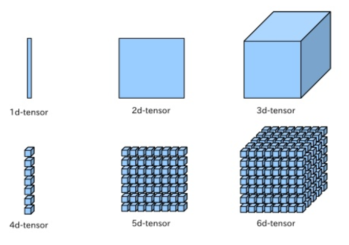
Tensors⌗
Tensors are a general name for multidimensional data. A 1d tensor is a vector, a 2d tensor is a matrix, a 3d tensor is a cube, a 4d tensor is a vector of cubes, and so on.
PyTorch mostly defines and speaks tensors:
X = torch.tensor([[0, 0], [0, 1], [1, 0], [1, 1]], dtype=torch.float32)`
Defining neural networks in PyTorch is about specifying the shapes of tensors for the neural network architecture you want to build.
A 2D image as data, can be represented by a (row, column, channel) tensor of pixels, where channel is the RGB channel for color:
image = torch.tensor([768, 1024, 3], dtype=torch.uint8) # uint8 pixel values between 0 and 255
Tensors become important when we get to the part on training using batches, GPU acceleration and performance optimizations.
PyTorch Models⌗
Given:
class XORNN(nn.Module):
    def __init__(self):
        super(XORNN, self).__init__()
        self.fc1 = nn.Linear(2, 2)  # Input layer with 2 neurons (for 2 input features)
        self.fc2 = nn.Linear(2, 1)  # Output layer with 1 neuron (for 1 output)
        self.relu = nn.ReLU()  # Activation function
Peeking under the hood of self.fc1, reveals tensors that capture the current weights:
model.fc1.weight
> tensor([[-0.2161, -0.4656],
         [-0.3299,  0.2059]], requires_grad=True)
And the calculated gradients/derivatives of error from the backward pass in:
model.fc1.weight.grad
>
tensor([[-3.5395e-03, -1.9939e-03],
        [ 2.3395e-05, -8.5202e-04]])
Activation results/metadata are created on the forward pass (as they’re needed for computing gradients), then thrown away. Calling model.eval() and/or torch.inference_mode() disables capturing activation results as they’re not required to be stored for inference.
As these networks get really large, optimization libraries (talked about in later sections) fudge with the precision of these weights, gradients and activations, and deal with moving them around efficiently - from GPU to DRAM to NVRAM etc. As an foreshadowing example: the bitsandbytes library is a drop-in wrapper around CUDA functions to enable 8-bit optimizers, matrix multiplication and quantization.
Acceleration of Training and Inference⌗
First, an exploration of CPU architecture to give a sense of relative difference between traditional computation and parallel/vectorized computation.
CPU⌗
-
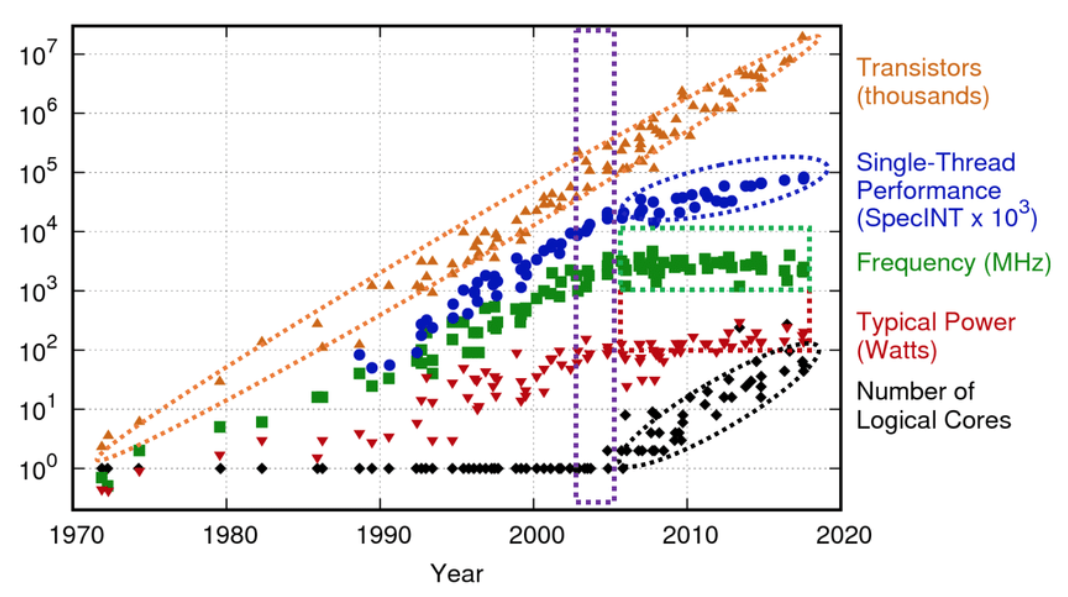
CPU architecture and performance over time:
-
SISD (single instruction, single data) and SIMD (single instruction multiple data).
-
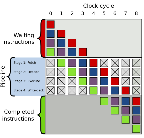
Pipelined execution (Scalar Pipelined Execution). Instructions and data are read from memory (typically employing read-ahead performance strategies) and streamed into the CPU’s execution pipeline:
-
Many optimizations employed to re-arrange that pipeline of instructions for performance. Instruction parallelism (Superscaler execution: executing multiple independent instructions in parallel), thread parallelism (hyper-threading etc), instruction re-ordering, loop unrolling etc. to improve throughput of instruction streams.
-
On-die caches (L1, L2, L3 and occasionally L4) employed to speed up instruction and data retrieval:
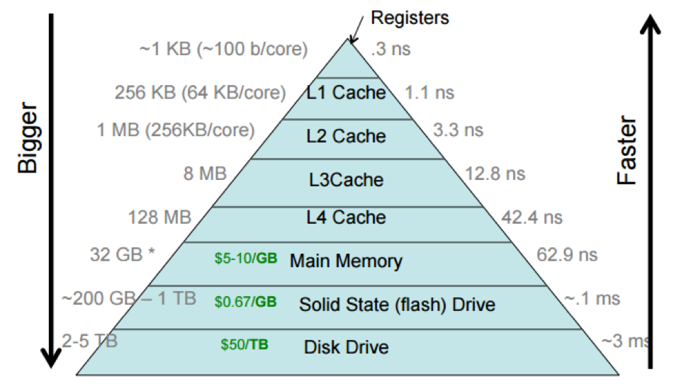
- Cache size and latency chart above is a bit old. Latest 13th gen consumer Intel chips have ~36MB L3’s. L4 is uncommon.
- AMD EPYC has up to 256 hardware threads, and up to 1.1GB of L3 cache at a TDP of 400W.
- Cache memory L3+ transfer rates are order ~400 GB/s
- DRAM transfer rates ~40-50GB/sec
- Specialized extended instruction set for floating point operations: AVX256 and AVX512 Advanced Vector Extensions.
- EPYC 7742 (128 threads, 3.4 GHz, 256MB L3 Cache) can do a theoretical 2.2 TFLOPS/sec double precision on AVX256 (source). Xeon 8380 seems to be able to do just over 3 TFLOPS/sec of double precision on AVX512.
GPU⌗
-
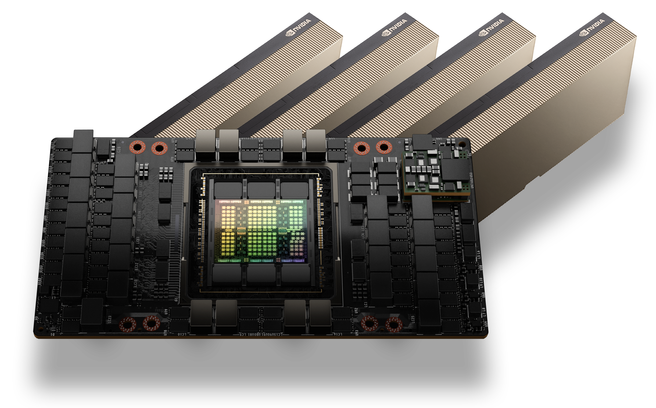
H100 is the latest NVIDIA GPU for deep learning workloads. Shown below are two form factors: PCIe (brown rectangular thing, and SXM which is the black circuit board).
-
SXM is a high bandwidth socket that connects NVIDIA GPUs to the board. ~700W of power delivery straight to the card (no cables required). 4-8 GPU slots.
-
30 TFLOPS @ FP64 (apples to CPU apples); 60TFLOPS @ FP32 and 2000 TFLOPS @ bfloat16.
-
3072 GB/sec memory bandwidth to 80GB of HBM3.
-
NVLink GPU interconnects (i.e. connecting GPU direct to GPU, any-to-any) can achieve 900 GB/sec on SXM and ~600GB/s on PCIe. You can think of NVLink as a supercharged PCIe.
-
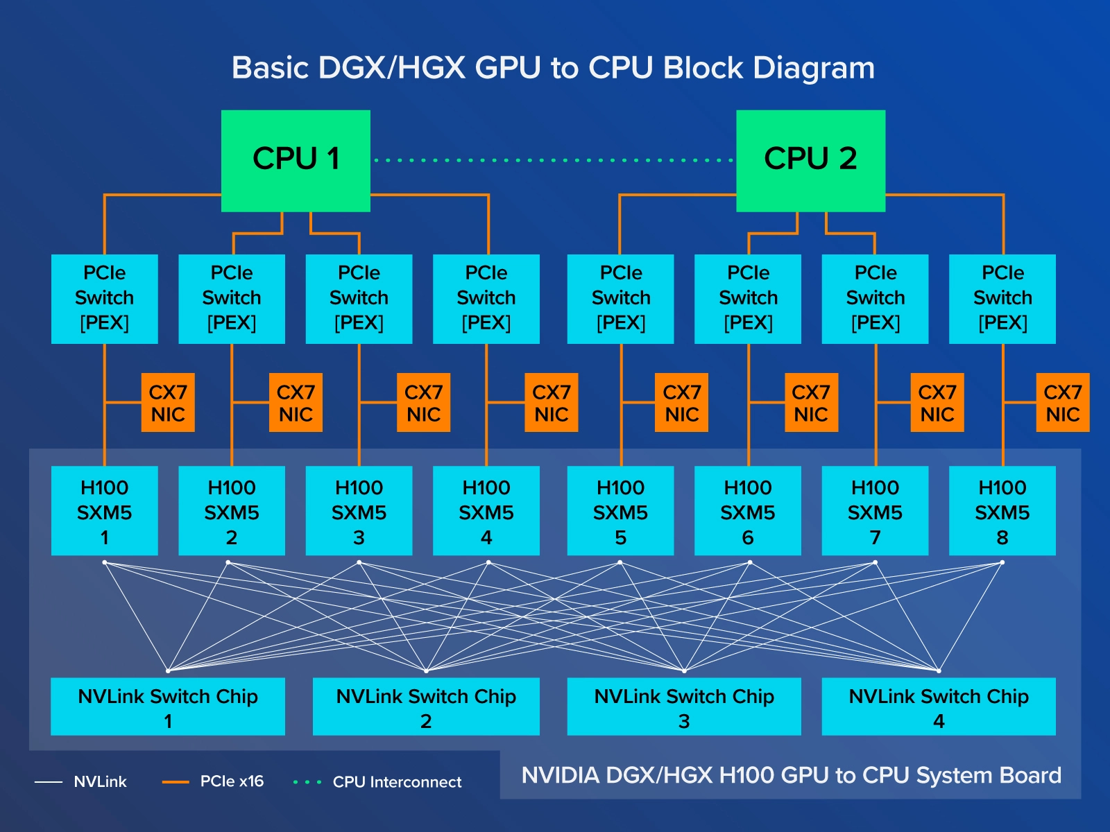
Configuration of 8 GPU with NVIDIA HGX baseboard with 2x CPU:
-
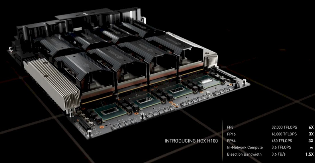
With a fully loaded HGX board stacked with 80GB H100’s, you’ll get:
- 16 petaFLOPS of FP16
- 640 GB of HBM3 memory
- 900 GB/s of intra-GPU bandwidth
- Total aggregate bandwidth of 7.2 TB/sec.
-
DGX is the name given to the pre-built 14’inch high rack mounted server you can buy.
-
NVLink GPU to GPU interconnect. Think of it as a significantly faster and higher bandwidth PCIe. Coherent data and control transmission over GPUs, but is also supported by CPUs. (One random fact, IBM used NVLink for CPU to CPU comms for POWER9).
-
NVLink and NVSwitch and how all that works is a bit confusing, so:
Networking⌗
- NVLink is a supercharged GPU to GPU signal interconnect. Just like a desktop computer with your classic AMD CPU has a specific number of PCIe ’lanes’ (AMD Ryzen 7000 series has 28 PCIe lanes supporting PCIe 5.0 bandwidth speed), a HGX board has a specific number of NVLink lanes.
- H100 has 18 fourth generation NVLink interconnect lanes, 900 GB/sec bandwidth.
- NVSwitch. NVLink connections can be extended across more GPU nodes and across machine boundaries to create a flat address, high-bandwidth, multi-node GPU cluster (like forming a data center-sized GPU).
- NVSwitch is an ASIC that connects to, and switches NVLink GPU to GPU communication.
- You can add a second tier of NVLink switches for cluster to cluster NVLink communication. NVLink second-level can connect up to 256 GPUs $( 32\space \text{machines} \times 8\space \text{GPUs})$ and 57.6 TB/s of all-to-all bandwidth.
- Going beyond 256 GPU’s requires hitting the network, so we have to head out via PCIe through a physical network interface, enter Infiniband:
- Infiniband (details about ConnectX-7, the latest here) is an NVIDIA aquired networking standard (think of it like a faster, higher bandwidth, lower latency Ethernet) through its acquisition of Mellanox.
- Infiniband defines the protocol, switching and signaling, physical materials (optics up to 10km) and higher level message passing/software API.
- Network Adapters for Infiniband perform two amazing feats:
- They do 400 Gb/sec.
- They do RDMA (Remote Direct Memory Access), which allows the network adapter to ‘zero copy’ data from GPU memory straight to the wire, bypassing the CPU. Recipients can do the same, where the network adapter will push inbound straight to GPU memory.
- Thus, 256 GPU’s NVLink via NVSwitch, or > 256 GPU’s via Infiniband connections between “pods”.
SuperPODs⌗
-
NVIDIA DGX SuperPOD is basically that 256 GPU cluster:
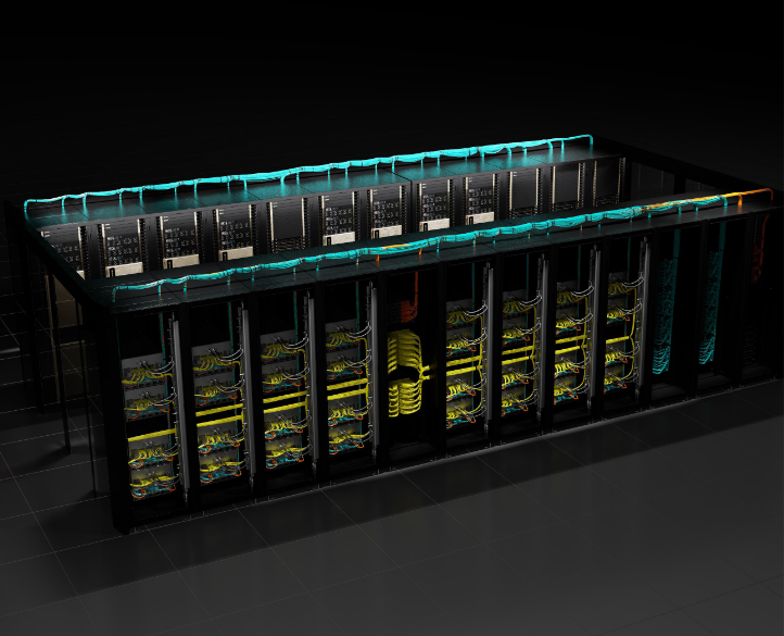
-
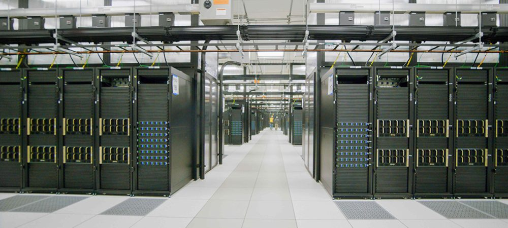
Facebook has the Research Super Cluster which has ~6080 GPU’s via 760 NVIDIA DGX A100 systems, and ~56 Petabytes of storage and connected via Infiniband.
Why so much compute, memory and bandwidth?⌗
- Generally hard to find good documentation and papers on the compute, memory and networking requirements for training the largest models around today, but we can estimate:
- GPT 3 (175 billion parameters), trained at float16 precision.
- ~650 GB for weights, ~650 GB for gradients, roughly 650 GB for the intermediate activations, and another ~650 GB for optimizer states (gradient statistics and so on).
- Roughy 2.7 TB of memory required.
- A SuperPOD of 256 80GB GPUs gives you ~20 TB of HBM3 memory, enough to train GPT.
- Rumor has it GPT 4+ is ~1-2 trillion parameters.
Significant amount of optimization work needs to be done to efficiently package and train these large models. Might explore some of these later, via papers like this one.
GPU in the small⌗
TODO: how GPU’s work
- GPCs (GPU Processing Clusters)
- SMs (Streaming Multiprocessors)
- CUDA cores
- Tensor cores
- shared memory, L1/L2 cache
- building cuda kernels
H100 Physical Architecture⌗
| H100 SMX5 | A100 SXM4 | |
|---|---|---|
| SMs | 132 | 108 |
| FP32 CUDA Cores Per SM | 128 | 64 |
| FP64 CUDA Cores Per SM | 128 | 32 |
| Tensor Cores | 528 | 432 |
| L2 Cache Size | 50MB | 40MB |
| TDP | 700W | 400W |
-
Physical layout of the H100: GPCs, SMs, Cores, Cache, HBM3, and PCIe interface:
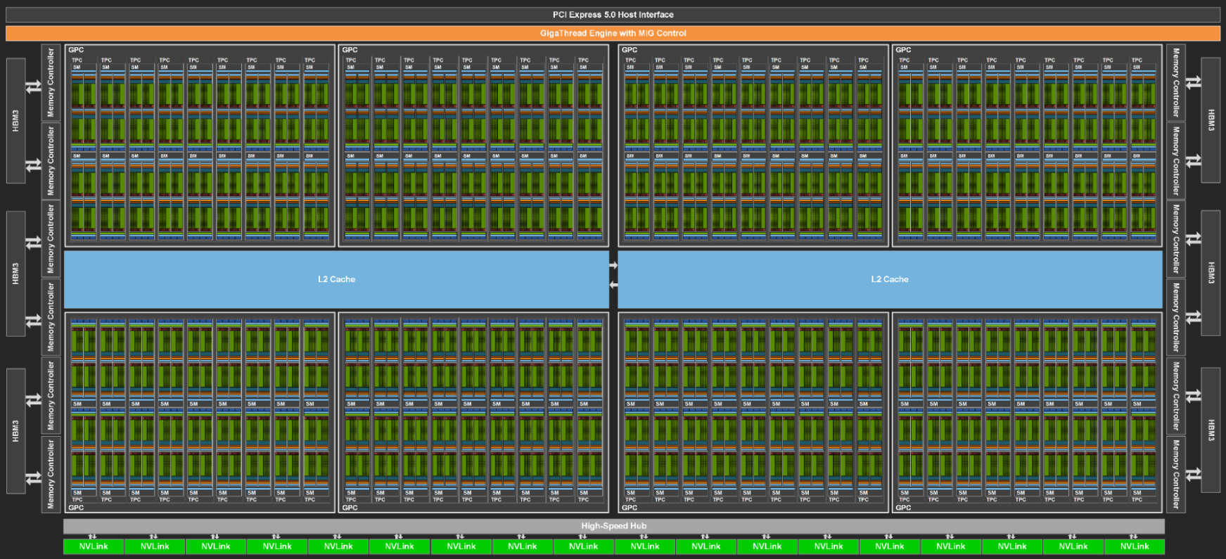
-
GPU Processing Cluster (GPC): A physical grouping of SMs. Hardware accelerated barriers, and intra-GPC data sharing for SM to SM communication. GPCs can be programmatically accessed, and form a nice logical grouping for programmers to access beyond typical SM programming. Clusters are a H100 feature.
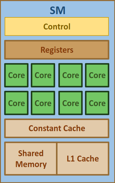
-
Streaming Multiprocessor (SM): Fundamental logical (and physical) processing unit in NVIDIA. Houses the compute cores, schedulers, load/store units, L1 cache, Shared Memory.
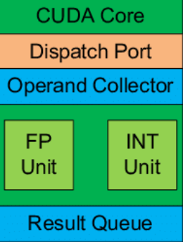
-
CUDA Core: processing elements within SM. Executes FP/INT instructions. Older architectures can do 2x FP or 1x PF and 1x INT instruction in parallel. Not sure what H100 can do.
-
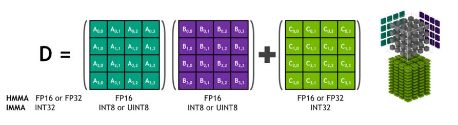
Tensor Core: processing element for tensor calculations. Mixed precision, although not all precisions are supported. H100 turned off some precisions, and turned on others. Previous generations of NVIDIA GPU could do 4x4 tensor calculation, but I think A100/H100 can do 4x8.
-
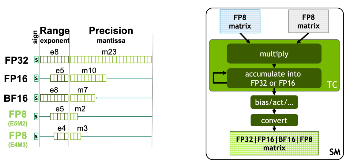
Inside the H100 Tensor core, with an example of FP8 matrix multiplication and accumulation:
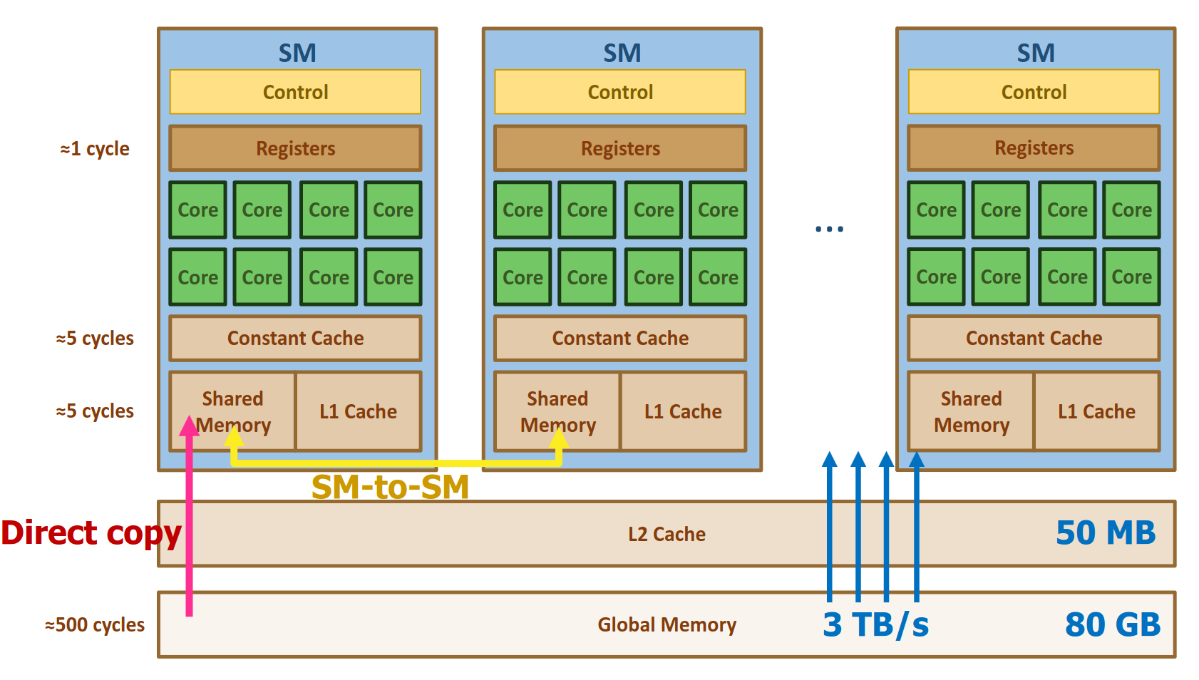
- Memory access layout of an NVIDIA GPU, the sizes of caches and memory, and the throughput and latency of memory access. The diagram below also shows a high level view of how memory is accessed and shared between Streaming Multiprocessors:
-
Memory and execution semantics are programmed using a “logical” grouping and scheduling system that maps reasonably well to the physical hardware groupings we see above. These logical grouping and scheduling primitives (foreshadowing: Clusters, Blocks, Warps, and Threads
-
CUDA Kernel: a function that is executed on a CUDA enabled NVIDIA GPU. You can think of CUDA as more like a low level programming API. There are methods that deal with the logical aspects of GPU programming (talked about later) like scheduling, threads, blocks, and so on, and the actual computation part: the mathematics applied to the data flowing through the CUDA cores. CUDA is an API and an extension to the C++ programming language. The
nvcc(NVIDIA compiler) is used to build a C++ program that contains a CUDA kernel function. -
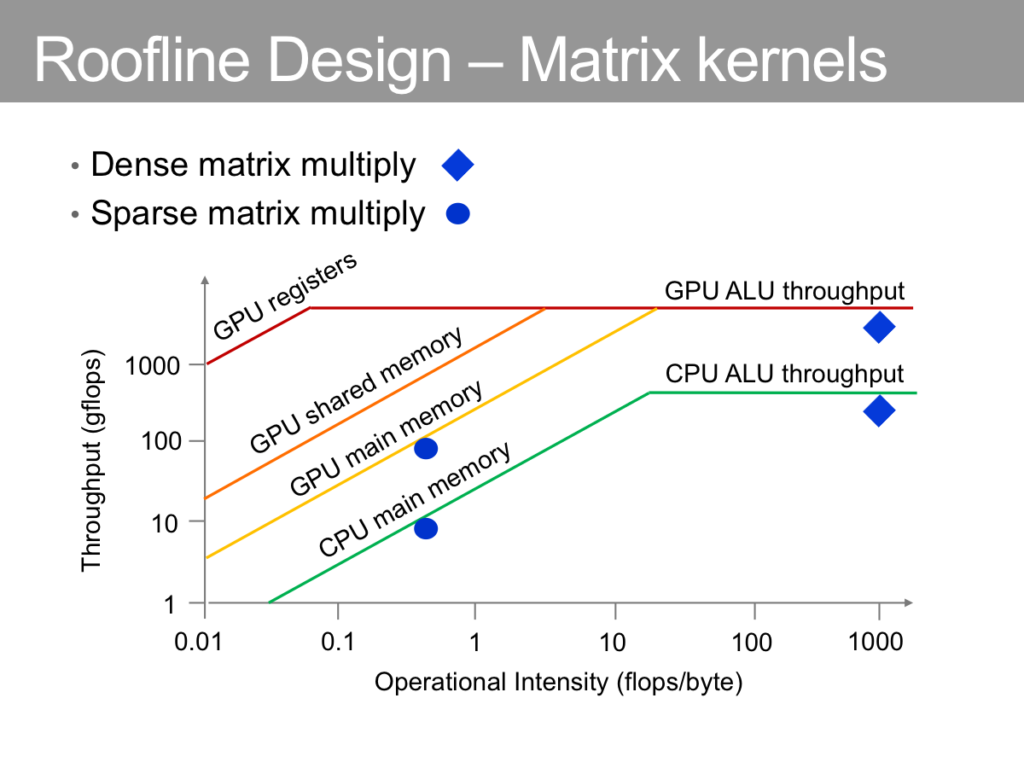
“Roofline” (or the ceiling of computing performance) of GPU relative to CPU via different memory mechanisms:
Talking about the logical aspects of GPU programming means we have to take a quick look at the CUDA API and programming abstraction:
“My first matrix multiplication” CUDA routine:
#include <iostream>
#include <cuda_runtime.h>
#include <cmath>
#include <chrono>
#include <cublas_v2.h>
#include <cblas.h>

__global__ void myMatMulKernel(float* A, float* B, float* C, int N) {
    int row = blockIdx.y * blockDim.y + threadIdx.y;
    int col = blockIdx.x * blockDim.x + threadIdx.x;

    if (row < N && col < N) {
        float val = 0.0;
        for (int i = 0; i < N; ++i) {
            val += A[row * N + i] * B[i * N + col];
        }
        C[row * N + col] = val;
    }
}

int megabytes = 50
int N = static_cast<int>(sqrt((megabytes * 1024 * 1024) / (sizeof(float))));

// ...

dim3 threadsPerBlock(16, 16);
dim3 blocksPerGrid((N + threadsPerBlock.x - 1) / threadsPerBlock.x,
                   (N + threadsPerBlock.y - 1) / threadsPerBlock.y);

myMatMulKernel<<blocksPerGrid, threadsPerBlock>>(..., ..., ..., ...)
And while we’re doing the “hello world” of CUDA, let’s test the performance of it against cuBLAS and CPU cblas:
Device 0: NVIDIA GeForce RTX 4090
Matrix dimension: 3620 x 3620
Matrix size in megabytes: 49.9893 MB
Setting matmul to **myMatMulKernel**
Time for loop 0: 44.6998 ms
Time for loop 1: 43.1279 ms

Setting matmul to **cublas**
Time for loop 0: 32.2928 ms
Time for loop 1: 26.7959 ms

Setting matmul to **CPU cblas**
Time for loop 0: 126.717 ms
Time for loop 1: 124.189 ms
CUDA, as a bunch of bullet points:
- Three main steps required to run a CUDA program:
- Copy the input data from host memory to device memory.
- Load the GPU program and execute, caching the data on the GPU for performance
- Copy the results from device memory back to host.
- Looking at our previous ‘hello world’ example:
__global__ void myMatMulKernel(float* A, float* B, float* C, int N) {
    int row = blockIdx.y * blockDim.y + threadIdx.y;
    int col = blockIdx.x * blockDim.x + threadIdx.x;
- The kernel takes pointers to A and B matrices, and the result C as well. ‘N’ is the dimension of the matrices (assumes square matrices for simplicity).
- The kernel calculates row and column indices for the current thread using its block and thread indicies (CUDA sets this up for all kernels).
    float val = 0.0;
    for (int i = 0; i < N; ++i) {
        val += A[row * N + i] * B[i * N + col];
    }
    C[row * N + col] = val;
- You can think of the code above performing a matmul on a small piece of the larger data, with N, and the block and thread indexes setting up the boundaries for that data.
- The configuration of how big and how many of those smaller chunks of data comes later: Threads in a block get
  int megabytes = 50
  int N = static_cast<int>(sqrt((megabytes * 1024 * 1024) / (sizeof(float))));

  dim3 threadsPerBlock(16, 16);
  dim3 blocksPerGrid((N + threadsPerBlock.x - 1) / threadsPerBlock.x,
                     (N + threadsPerBlock.y - 1) / threadsPerBlock.y);

  // call our fancy matmul
  myMatMulKernel<<<blocksPerGrid, threadsPerBlock>>>(d_A, d_B, d_C, N);
- For a matrix of 50 megabytes @ sizeof(float)
Nwill need to be a matrix size of 3620x3620. - We define a 2D grid of threads, where each dimension has 16 thread, 16x16 = 256 threads, per block.
- With
Nbeing 3620 and a 16x16 thread block size, number of blocks ends up being 227 x 227 = 51529 blocks. - CUDA blocks are logical, not physical. They get mapped to a Streaming Multiprocessor (SM) via the CUDA runtime. The scheduler will try and fill up the SMs with as many thread blocks as possible. Each SM has at least 2 “warp schedulers” (I think H100 has four?), and a warp is a funny name for a group of 32 threads. Therefore, your thread blocks get mapped to warps which get mapped into SMs via the warp scheduler.
- When you launch a kernel, you specify a logical organization of your data, grouping threads into blocks, and blocks into a grid. CUDA maps this on to the physical hardware: into SMs, then onto warps, which then run those 32 threads in SIMT (Single Instruction Multiple Thread), but on different data.
- Physical mapping requires optimization: if you remember, SMs are grouped physically into GPCs, so intra-SM communication/data sharing will have differing latencies depending on grouping proximity.
Warp Branching⌗
- If threads within a warp take different paths due to conditional branching, the scheduler will execute these paths serially, disabling one side of the path at a time. This reduces throughput performance.
Speeding up things in the small⌗
Lots of libraries get built to optimize kernels for different shapes, sizes and precisions on both GPU and CPU:
Calling kernels from the CPU also has overhead: around 20-40 microseconds, so ping ponging between the CPU and GPU shuffling data and results back and forward will accumulate this overhead. You can hopefully enqueue enough kernels so that the GPU spends most of its time executing and not waiting between steps.
Spotting gaps in a GPU profile where the GPU is idle waiting for the host gives the dev a hint that optimization will be necessary:
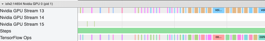
This can mean things like:
- Concatenating small tensors or using a larger batch size to make each launched kernel do more work.
- Switching away from “eager mode” to “graph mode”. Eager mode launches and runs operators (generally kernels) as soon as they’re seen; Graph mode builds an execution graph lazily, which is then compiled and executed on the GPU as a whole.
- Enabling backend kernel/graph optimizers like XLA, or TorchDynamo + Torch FX which crawl these execution graphs and perform optimizations on them like kernel fusion (taking multiple kernel calls and transforming them into a single kernel call).
Hyperparameters of GPU Optimization⌗
Hyperparameters are the ‘knobs and dials’ of an algorithm that determine the performance: training, inference, and model performance. The process of tuning these parameters for optimal performance is called hyperparameter tuning.
You can think of the physical hardware characteristics and the logical software parameters as “hyperparameters” for GPU tuning and optimization:
- Num of threads per block
- Blocks per grid
- Locality of code to shared memory
- Optimal use of registers for instruction throughput
- Memory access patterns
- Thread synchronization
- Precision
- Instruction mix (different instructions have different latencies)
- etc etc.
In the context of deep learning, you have logical groupings of data (weights) and logical groupings of matmul and other functions (forward pass and back-propagation) with order ~billions of data points that need to be mapped on to these GPUs via these hyperparameters. Mapping these well can mean orders of magnitude better training and inference performance.
The mapping is a bin packing problem which is considered NP-hard, where containers (the underlying neural net) with fixed sizes are provided and the goal is to find the best way to pack them into the GPUs physical boundaries.
Optimizations for Training and Inference⌗
Most of the ‘global’ model optimizations for training and inference are about multi-GPU multi-machine parallelism. We’ll go through the different types before looking at the libraries that offer support for them:
Parallelism⌗
(A lot of this is lifted/based on an old version of the HuggingFace parallelism docs
Different types of Model Parallelism, which can be combined (and this is basically what DeepSpeed does):
-
DataParallel (DP). Replication of weights, activations, embeddings etc across GPUs, and input data is sliced and sent through the replicated pipelines. Synchronization happens at the end of the pipeline.
-
TensorParallel (TP) or Tensor Slicing, or “Model Parallelism”. Tensors (weights) are split into multiple chunks across GPUs. Aggregations of full tensors happens only for operations that require it.
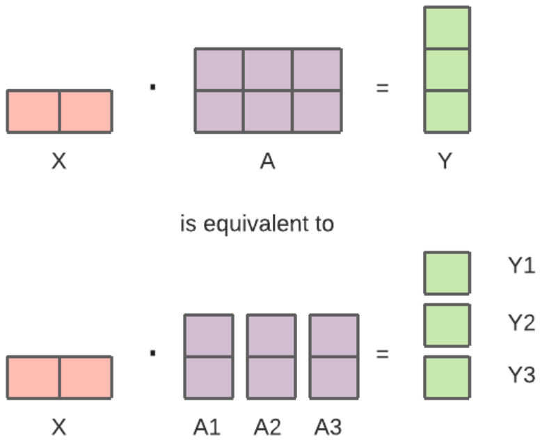
- HuggingFace docs point to a model example that benefits from TP in one of the Megatron papers:
-
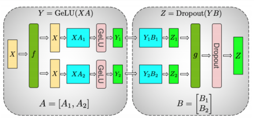
In this instance,
Ygets tensor slice parallelized over multiple GPUs as input intoGeLUforGeLU(X A)can be fed independently:$$ [Y_1, Y_2] = [ GeLU(X A_1), GeLU(X A_2)] $$
-
Where
Ais the split tensor weights, andXis the input data.dropout(Y B)requires the full tensorYwhich is were recontruction will happen.
-
PipelineParallel (PP). Weights are split up ‘horizontally’ (i.e. horizontal across layers, as they’re normally diagrammed) across GPUs and data is fed-forward across GPU boundaries.
- Input data is split into ‘mini batches’ to build a pipeline (in this diagram, the pipeline is going from the bottom to the top, with
Fbeing the forward pass andBbeing the backward pass:
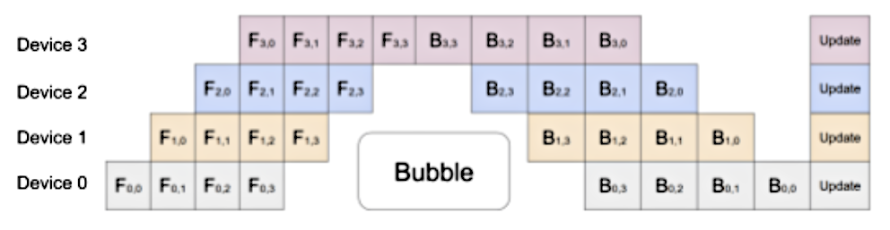
- The pipeline is then fed-forward across multiple GPU boundaries, however this creates a ‘bubble’ of idle work like the one seen above (albeit a smaller bubble than if a single batch was forwarded through).
- There’s a mini-batch parameter that you can tune to reduce the bubble size.
- HuggingFace has support for pipelining:
which will load a task specific pipline for a given model and take care of multi-GPU pipelining. The library
from transformers import pipeline generator = pipeline(task='automatic-speech-recognition')parallelformersperforms this optimization for HuggingFace transformer models.
- Input data is split into ‘mini batches’ to build a pipeline (in this diagram, the pipeline is going from the bottom to the top, with
The techniques discussed are combinable, which is what libraries like DeepSpeed (mentioned next) help you do:
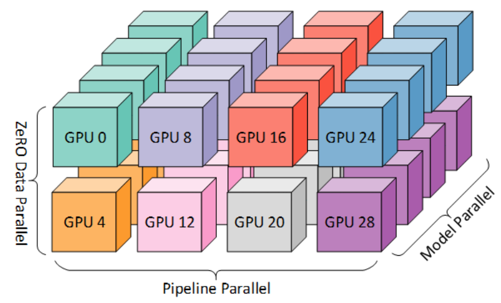
(mapping of workers to GPUs on a system with eight nodes, each node has four GPUs. Coloring denotes GPUs on the same node. Model Parallel here is synonymous with ‘Tensor Parallel’)
DeepSpeed⌗
Microsoft Research DeepSpeed (which is a palindrome!) notes. Speeds up both training and inference for PyTorch models, sometimes by orders of magnitude. It’s a wrapper on PyTorch.
Before diving in to the different optimizations and techniques, we should look at ZeRO first, as it’s kind of central to most of the DeepSpeed work. ZeRO (and I guess their latest stuff, ZeRO Infinity?) feels to me like a collection of techniques for training (and inference) scaling:
-
Infinity Offload Engine: makes GPU, CPU and NVMe memory sort of like a “flat address space”, where weights, activation’s, embeddings etc can live anywhere on those different memory types, sort of ‘opaque’ to the training and inference process. This means scaling model sizes well beyond available GPU memory.
-
Memory-centric tiling: TODO
-
Bandwidth-centric partitioning: TODO (although I think what this is doing is exploiting the fact that with NVLink and NVSwitch you can treat multiple GPUs on node and cluster as being “one”)
-
ZeRO-Infinity paper has the following diagram, which shows
Layer 0weights, calculated gradients and optimizer states being partitioned across DRAM + NVMe. These are loaded in parallel into multiple GPUs, gradients calculated and pushed back down and re-partitioned across DRAM NVMe: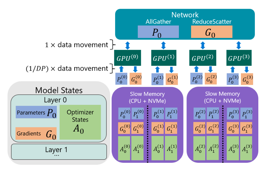
- One of the neat things explained in the paper is the requirement that NVMe/PCIe bandwidth be completely saturated - it takes into account things like a) parallelized reads from NVMe being desirable, b) the NVMe -> CPU -> GPU data transfer resulting in possible memory fragmentation, and c) overlapping reads/writes to NVMe etc etc. It looks like it optimizes memory block sizes and scheduling to achieve optimal and saturated throughput.
-
TODO: explain the rest of the paper
Inference⌗
- Multi-GPU parallelism. Partitioning models that are larger than single GPU VRAM across multiple GPUs. Introduces cross-GPU communication overhead, and can reduce per GPU computation granularity. There ends up being a latency/throughput trade-off as you’re deciding the parallelism ‘degree’ (i.e. how much parallelism). This “inference-adapted” parallelism is a tunable parameter within DeepSpeed.
- Supports Tensor Parallel tensor slicing based multi GPU parallelism for Transformer models, both within nodes and across nodes.
- ZeRO-inference
- Uses “ZeRO-Infinity” techniques applied to inference.
- Pins model weights in CPU or NVMe, and streams weights layer-by-layer in to the GPU for inference computation. Outputs are kept in GPU VRAM for next layer calculation.
- Inference time is GPU layer compute + PCIe fetch time.
- Very throughput orientated: by limiting GPU memory usage of the model to a few layers, ZeRO inference can use the majority of GPU memory to support a large amount of input tokens (long sequences or large batch sizes).
- One GPT3 175B layer requires 7 TFLOPS to process an input of batch size 1 and a sequence length of 2048. Computation time dominates over the latency of fetching model weights.
- Supports layer pre-fetching.
- Has this cute trick where GPUs will fetch a sliced tensor from multiple different PCIe links, then enable GPU-GPU higher speed data transfer via NVLink to have each GPU get the entire tensor. Super cute.
- TODO: finish
Training⌗
Speeds up training through: optimizations on compute/communication/memory/IO and effectiveness optimizations on hyperparameter tuning and optimizers
- As with inference, enables data parallelism, model parallelism, pipeline parallelism and the combination – I guess they call it 3D parallelism?
- Distributed training with Mixed Precision
- Uses “ZeRO” optimizer: data parallel, partitioning of model states and gradients across CPU/NVMe etc.
- 1-bit Adam optimizer reduces communication intra-node by up to 26x.
- Layerwise Adaptive Learning: an optimization strategy where different layers in the network might have different learning rates. DeepSpeed supports this as “advanced hyperparameter tuning”, via a sort of extension to Layerwise called LAMB
- Specialized transformer CUDA kernels.
- Progressive Layer Dropping: improves generalization performance of the network (reduce overfitting) and happens to be a performance improvement too. Layers get progressively “skipped” or “dropped” in the forward and backward pass of training. A few different strategies to this you can choose from.
- Mixture of Experts (MoE): build individual models that are trained on specific tasks or specific data (experts). Build a ‘gating network’ which is trained on figuring out what expert to route what request (i.e. for a given input space, what model should that input be sent to). During inference, the gating network directs each input to the appropriate expert for processing. The outputs of individual experts can be combined in a weighted sum to produce the final output.
- TODO: finish
NVIDIA TensorRT⌗
- NVIDIA TensorRT
- TODO: explain
OpenAI Triton⌗
- OpenAI Triton
- Python like programming language to build and deploy hardware agnostic kernels.
- Triton kernel for adding two matrices:
BLOCK = 512
# This is a GPU kernel in Triton.
# Different instances of this
# function may run in parallel.
@jit
def add(X, Y, Z, N):
   # In Triton, each kernel instance
   # executes block operations on a
   # single thread: there is no construct
   # analogous to threadIdx
   pid = program_id(0)
   # block of indices
   idx = pid * BLOCK + arange(BLOCK)
   mask = idx < N
   # Triton uses pointer arithmetics
   # rather than indexing operators
   x = load(X + idx, mask=mask)
   y = load(Y + idx, mask=mask)
   store(Z + idx, x + y, mask=mask)
- Python -> Triton-IR -> Triton Compiler -> LLVM-IR -> PTX (Parallel Thread Execution, assembly language for NVIDIA CUDA GPUs)
- LLVM IR:
def void add(
  i32* X .aligned(16),
  i32* Y .aligned(16),
  i32* Z .aligned(16),
  i32 N .multipleof(2)
) {
entry:
  %0 = get_program_id[0] i32;
  %1 = mul i32 %0, 512;
  %3 = make_range[0 : 512] i32<512>;
  %4 = splat i32<512> %1;
  ...
- PTX: CUDA Assembly:
.visible .entry add(
    .param .u64 add_param_0, .param .u64 add_param_1,
    .param .u64 add_param_2, .param .u32 add_param_3
)
.maxntid 128, 1, 1
{
    .reg .pred     %p<4>;
    .reg .b32     %r<18>;
    .reg .b64     %rd<8>;
    ld.param.u64     %rd4, [add_param_0];
    ...
- TODO: finish
Other Optimizers/Frameworks⌗
- FlexFlow - low latency high performance LLM serving.
- List of PyTorch Optimizers
- Apache TVM: End-to-end compilation stack for Machine Learning: unified IR (Intermediate Representation) that deep learning frameworks can lower down to, then that IR can be lowered down to GPUs, CPUs, ASICs and so on.
- Google XLA: XLA (Accelerated Linear Algebra). ML compiler stack for Tensorflow and PyTorch.
- Google JAX: Autograd (automatic differentiation library) + XLA (see above). Go from Python/Numpy to XLA to GPU/TPU.
- AMD HIP: C++ runtime and API to build GPU kernels for AMD /and/ NVIDIA GPUs. It’s basically AMD’s version of CUDA. HIPIFY is a tool to automatically convert CUDA code to HIP.
Large Language Models⌗
Transformer Architecture⌗
TODO
Training and Inference⌗
TODO
Local LLMs⌗
TODO
Fine Tuning⌗
TODO
Links⌗
- PyTorch memory tuning
- PyTorch tuning tips
- H100 Tensor Core GPU Architecture Whitepaper
- Heterogeneous Systems - GPU Memory Hierarchy
- GPU Programming basics
- Deep Learning Course
- vllm, efficient memory management for LLMs with PagedAttention, github
- A gentle introduction to torch.autograd
- AI Chips: A100 GPU with Ampere architecture
- How the hell are GPUs so fast?
- Understanding GPT tokenizers
- TPUs vs GPUs for Transformers BERT
- Implementing a Transformer from scratch in PyTorch